Verification of Clinical Plans
OCTAVIUS 4D and the Standard top were used for the verification of 46 clinical plans (mostly VMAT, some IMRT). The most frequent photon energies were 10X, 6FFF and 10FFF (12 plans each). The other energies were less frequent (6X: 9 plans, 15X: 1 plan).
All analyses were performed with both approaches for the TPS phantom. The first approach uses different structure sets for AAA (TPS Phantom I) and AXB (TPS Phantom II), whereas the second approach uses a single structure set for both algorithms (TPS Phantom III). The analysis of the second approach was done retrospectively: the measurement needs not be repeated - only the new cross-calibration factor has to be calculated. Then the measurement is compared to the calculation based on the "STD thin H2O" phantom.
If you have not read about our method of analyzing the measurements yet, this you should do that now.
Documentation of OCTAVIUS 4D QA Results
As with the Portal Dosimetry results, the OCTAVIUS 4D QA results are documented in iCheckNet:
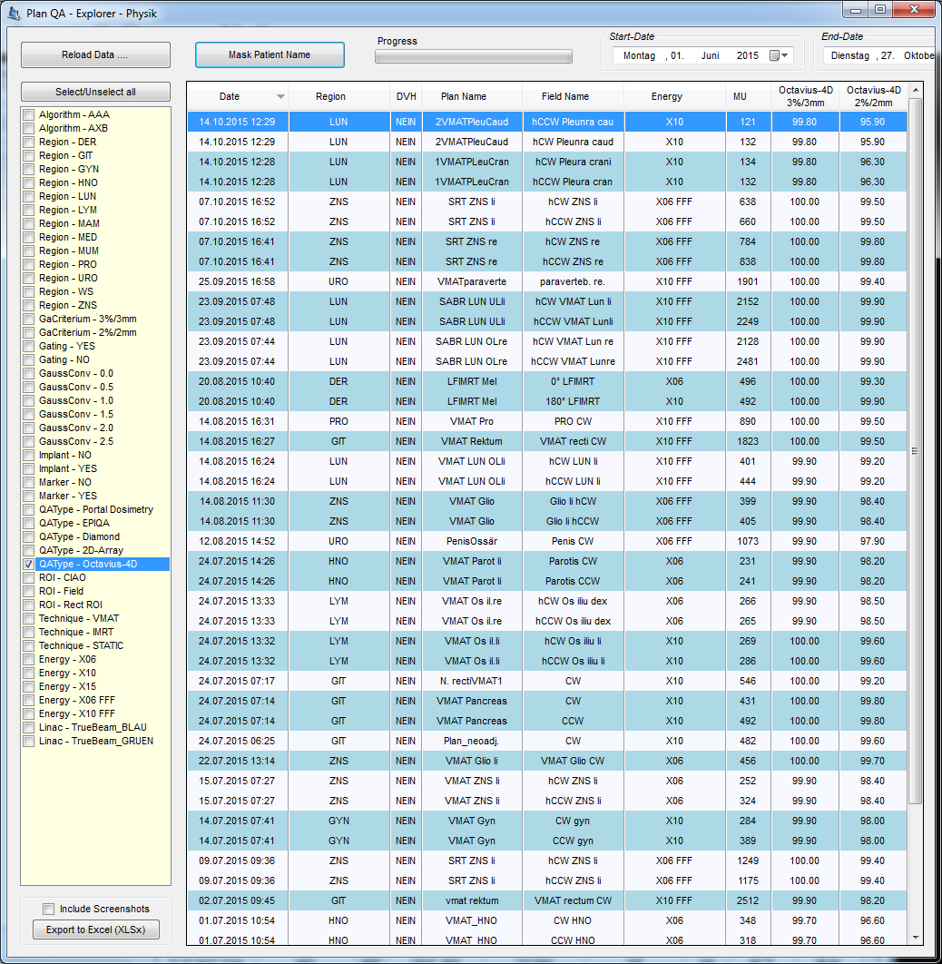
The last two columns contain the results of the 3G3 and 2G2 analysis. As already mentioned, a single number is not able to describe the 3D result. However, we did not want to create 20 more columns in the table, to document all the results for the individual dose levels. To get more information, a patient has to be double-clicked. This opens a view with all patient related QA results:
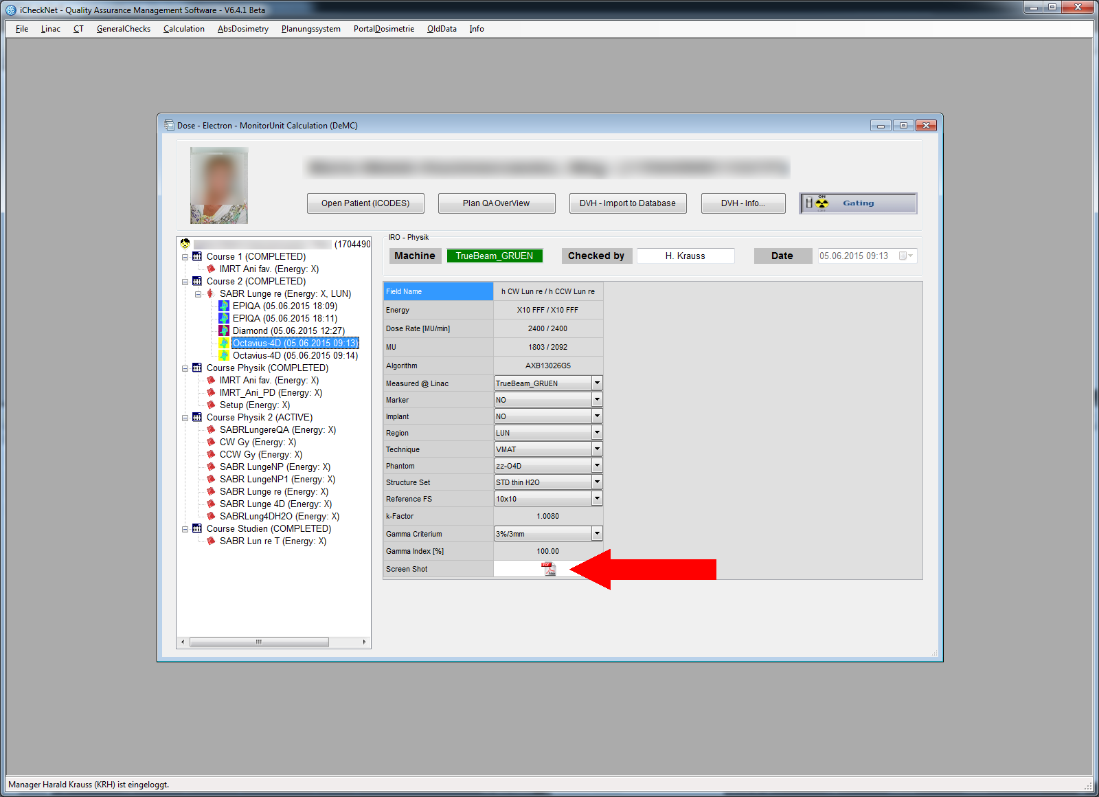
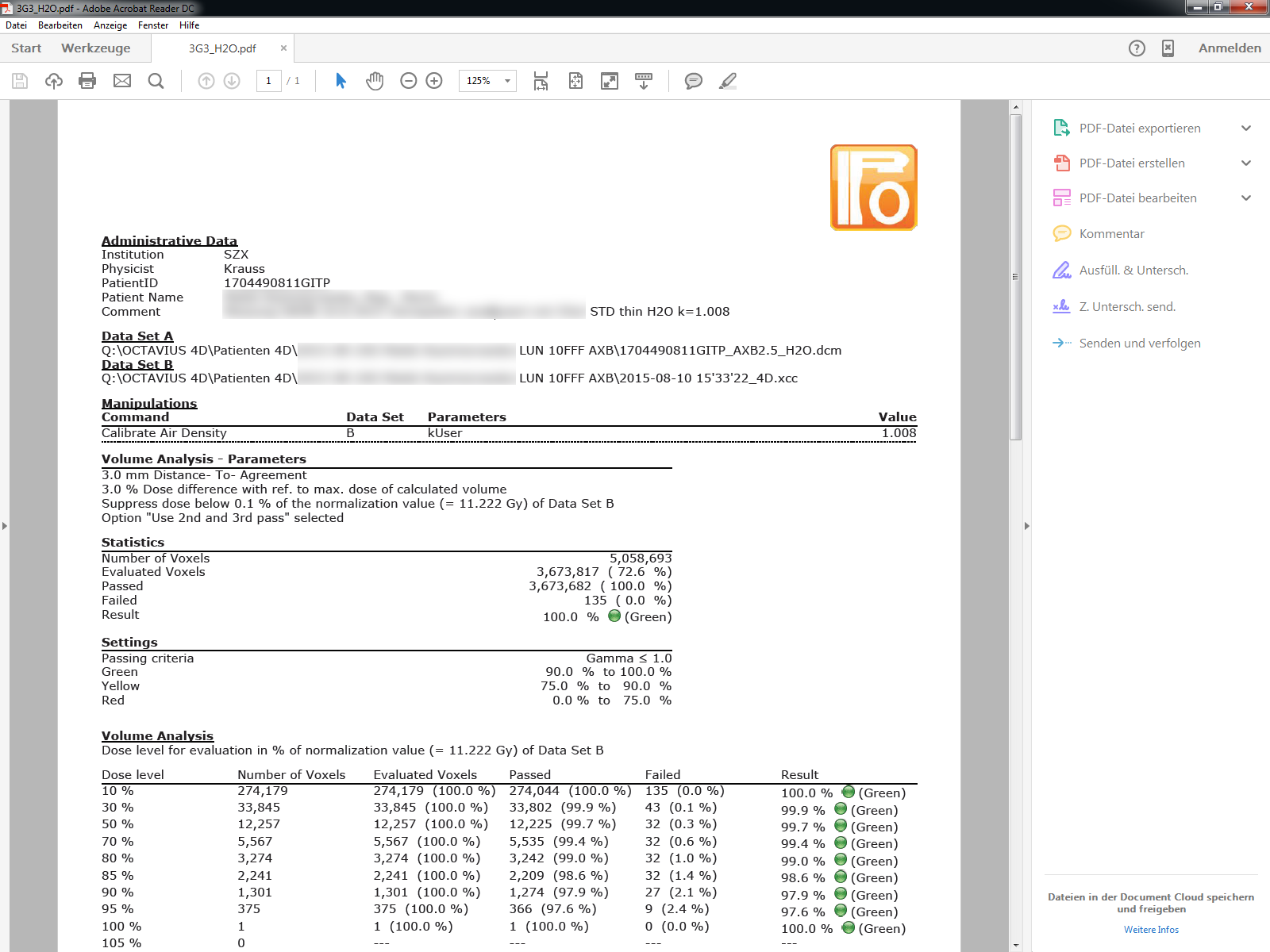
Clicking on the small PDF icon (red arrow) brings up the full VeriSoft report:
A technical detail: with Portal Dosimetry, we always measure field by field (arc by arc), whereas with OCTAVIUS 4D we usually measure the whole plan. Therefore, we do not get individual results for each arc, only one result per plan. In iCheckNet, the plan result is connected to each field, which is why in the overview, the OCTAVIUS 4D results for different arcs in the same plan are always identical.
AXB - Differences between Phantom II and Phantom III
For AcurosXB plans, TPS Phantom III gave slightly, but consistently better results than TPS Phantom II for all dose levels, from 10% to 95% of the normalization value.
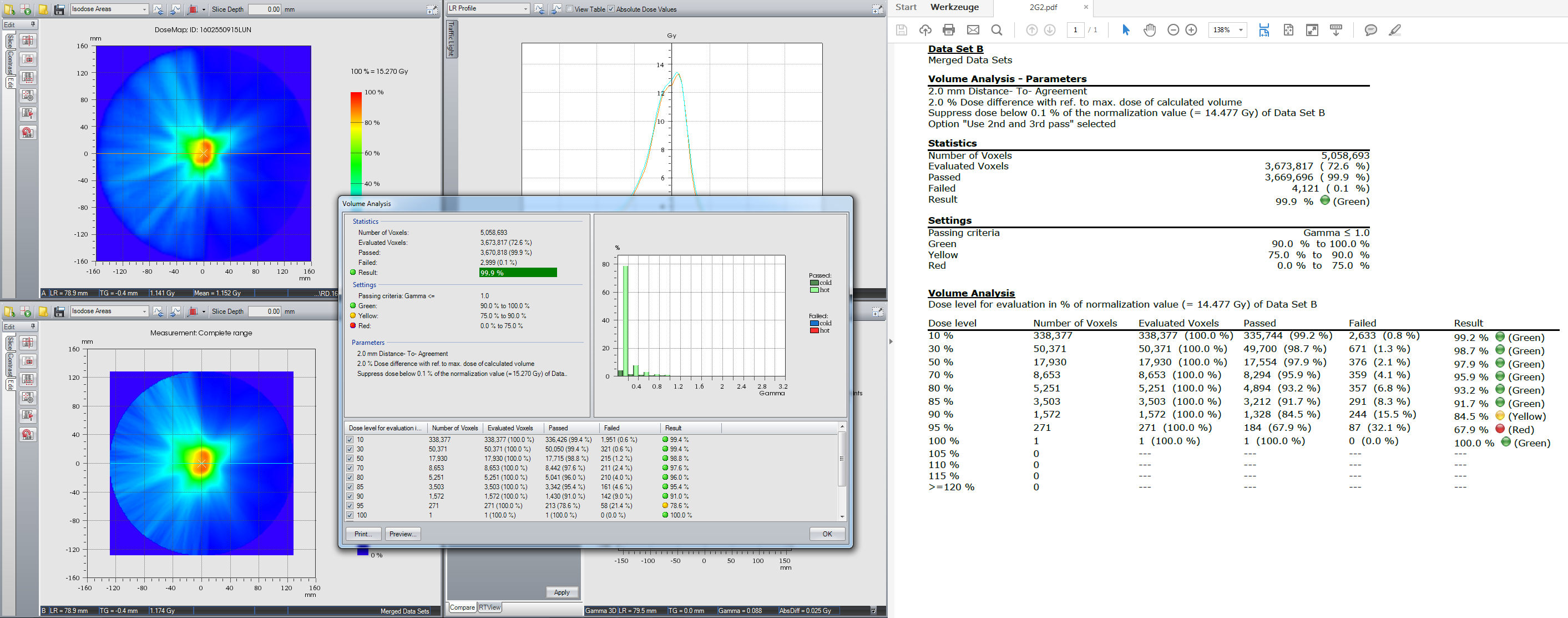
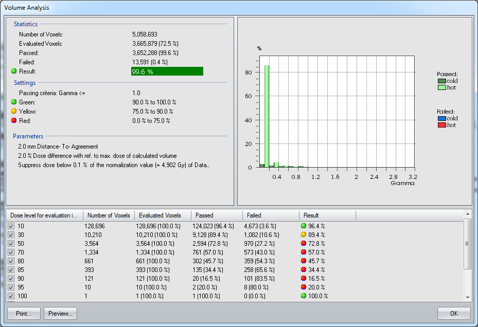
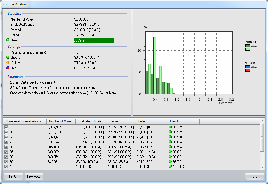
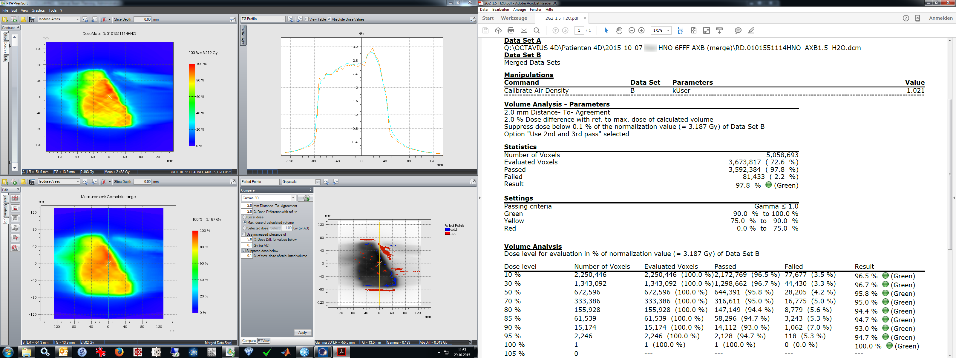
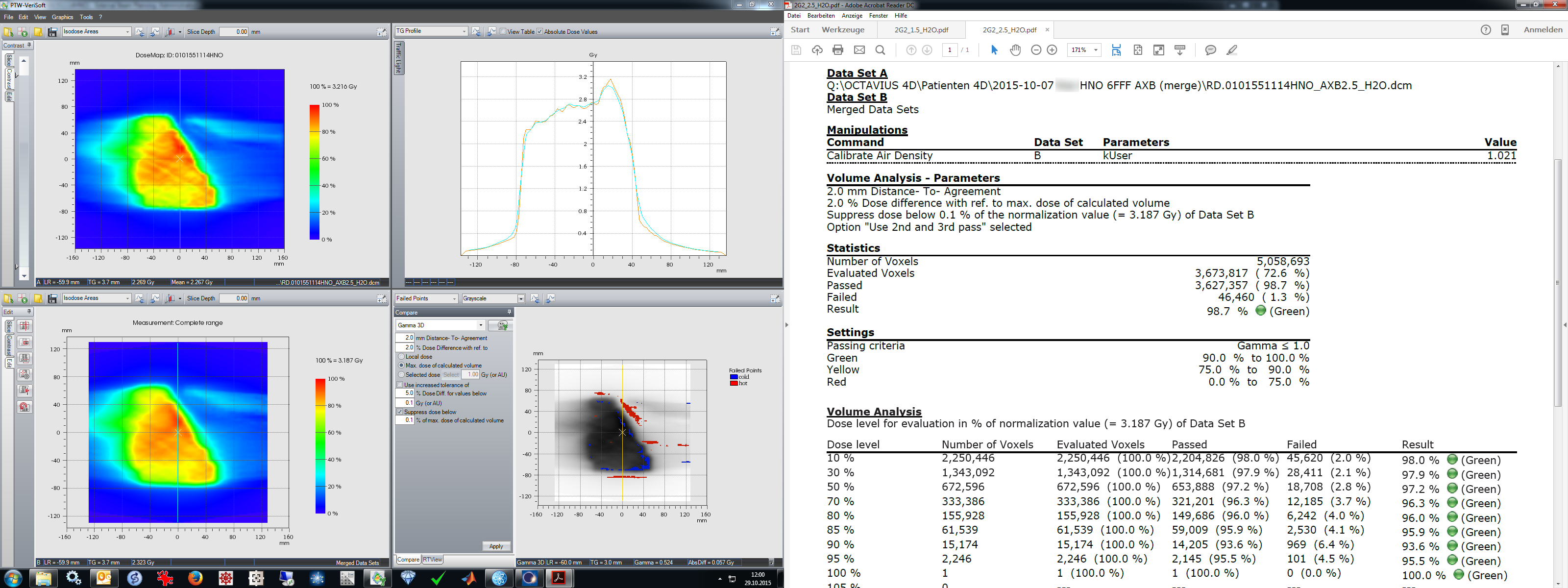
The improvement was typically around 1% in higher dose levels, but can even be larger. The following screenshot shows the volume analysis (Gamma 3D, 2G2) of a SABR lung plan (3 x 13 Gy to 95% of target volume), calculated with AXB. The right side shows the PDF report of the volume analysis based on the older Phantom II, the left side shows the retrospective analysis of the same plan based on the newer Phantom III. At the 95% dose level, the 2G2 result improved from 67.9% to 78.6% (10.7% improvement):
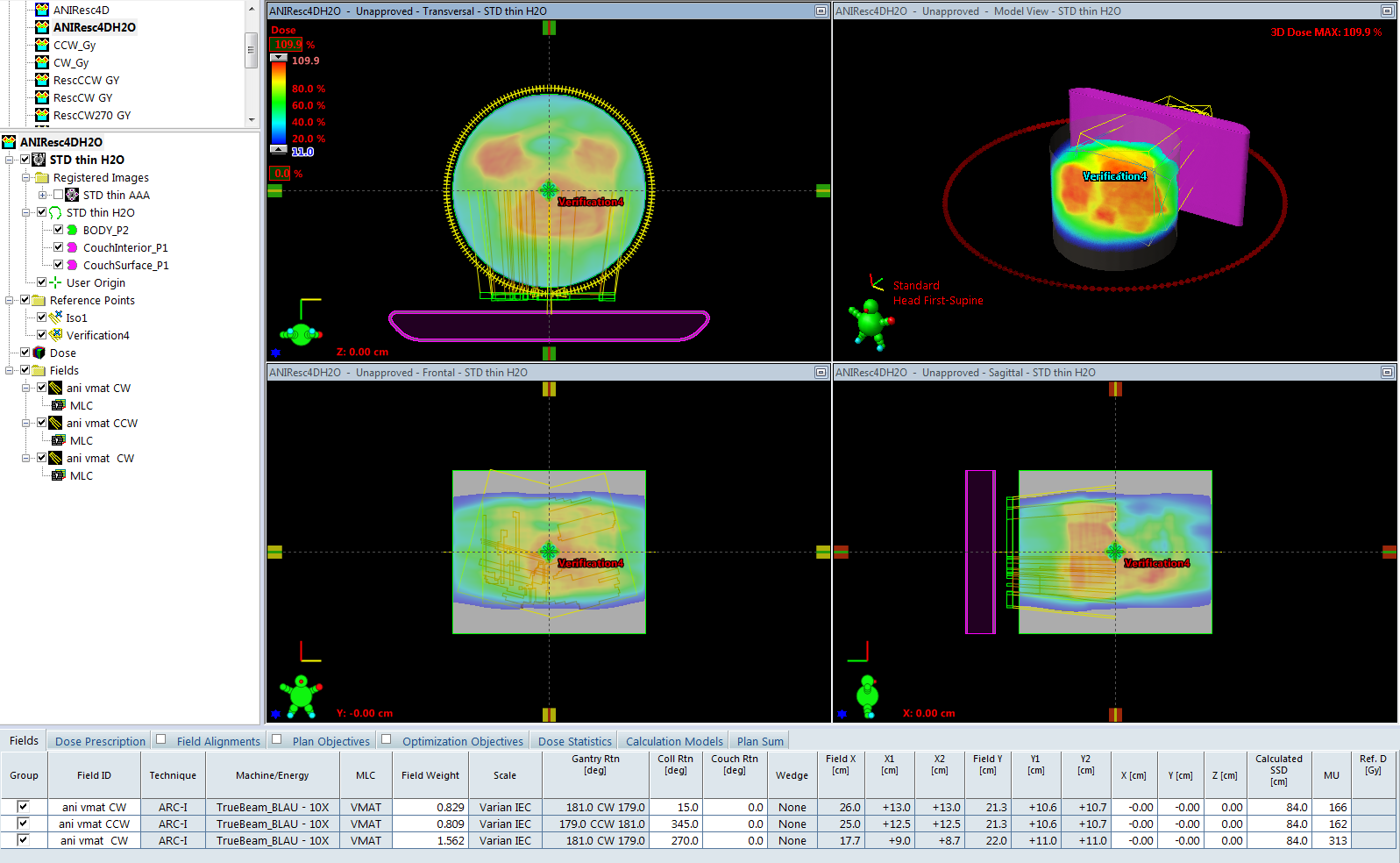
This was the corresponding clinical plan:
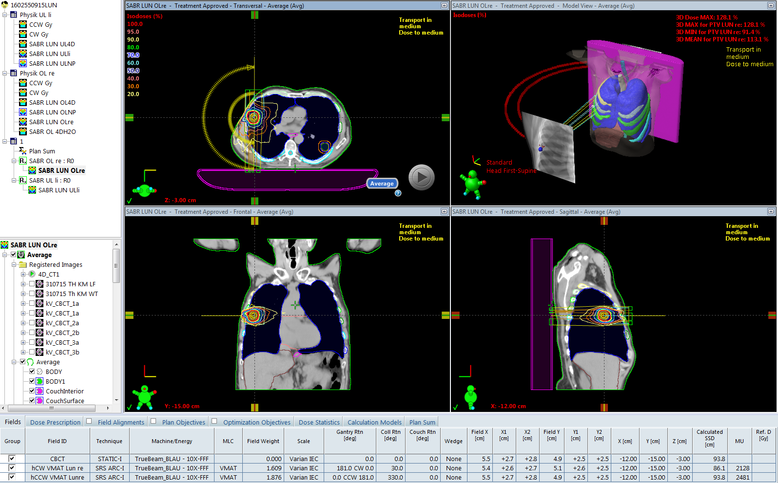
The switch from Phantom II (37 HU, polystyrene) to Phantom III (0 HU, water) increases both calculated and measured dose at isocenter. Calculated dose is higher because the material, as seen by Acuros, is less dense. Measured dose is higher, because the raw measurement is multiplied by a cross-calibration factor, k, and k is larger because the reference dose calculated on Phantom III is also larger.
For the above example (SABR lung plan), the maximum dose of matrix A due to the switch of phantoms increased from 15.334 Gy to 16.056 Gy, which is +4.71%. But the maximum dose in measurement matrix B (which VeriSoft takes as 100% dose level for the volume analysis) increased from 14.477 Gy to 15.270 Gy, which is +5.48%. A change in the max. dose leads to a rebinning of voxels.
One question remains: why don't the doses of matrix A and B increase by the same amount?
AAA - Differences between Phantom I and Phantom III
For AAA plans, the results of Phantom III and Phantom I were practically identical.
For convenience, we therefore choose Phantom III for verification, one TPS phantom for both AAA and AcurosXB.
Some Clinical Examples
We do not want to present here an extensive list of results as with Portal Dosimetry, but just one or two (dosimetrically) interesting cases.
Example 1 - Very Small Fields
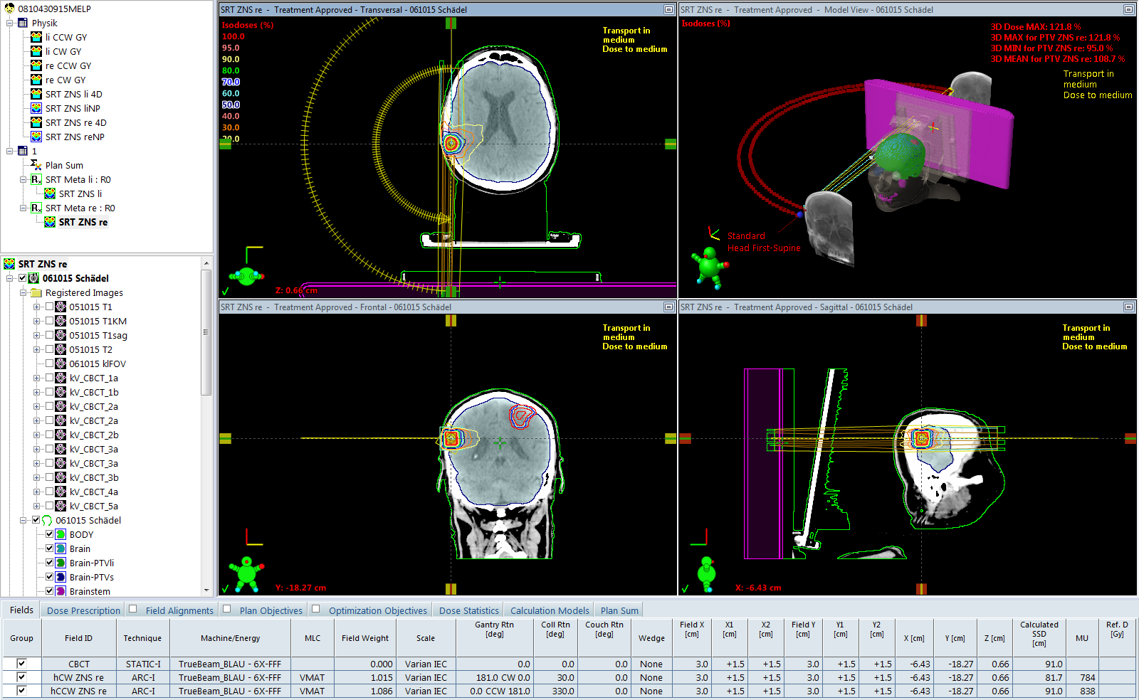
The first example belongs to the category of rather small arcs. It is the treatment of one of two metastases in the brain. Three times 8 Gy were delivered with 6FFF to 95% of the volume. The PTV on the right side of the brain (2.97 cm3) was about spherical, with an equivalent sphere diameter of 1.8 cm:
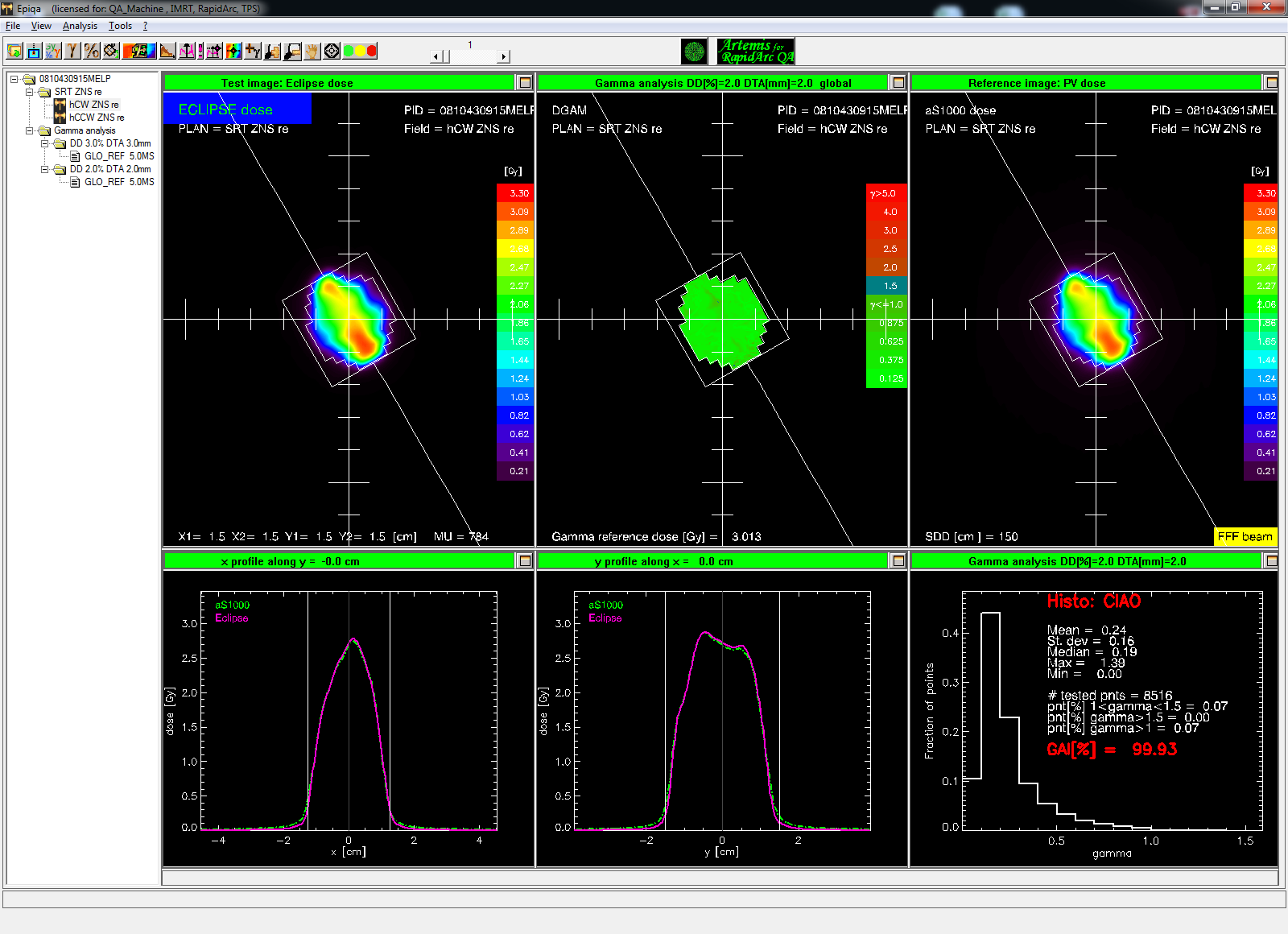
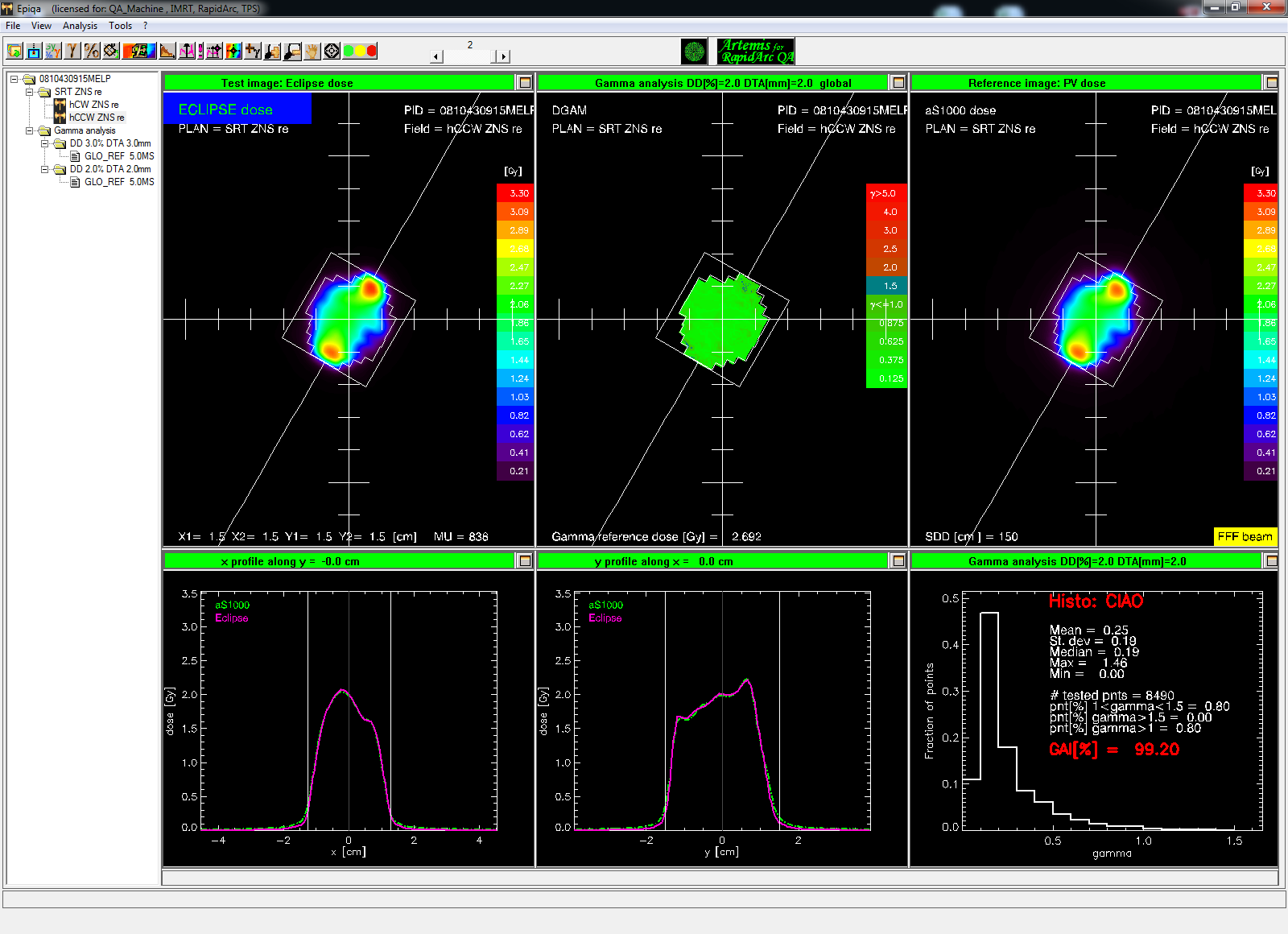
PTW offers a special 2D Array to verify such small fields, but we wanted to give it a try with our system. The EPIQA results for the CW- and CCW-arc and 2G2 were already sufficient, should the OCTAVIUS 4D result fail.
Due to the tiny field size, two measurements were performed, and merged.
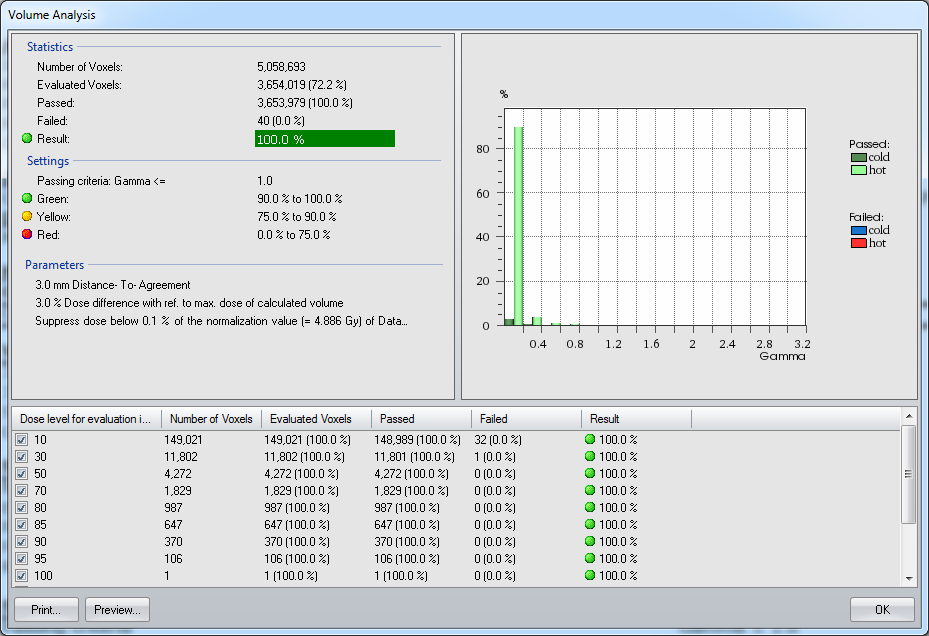
For 3G3, the VeriSoft results seem to be quite good. Peak dose is a little too small in the target center, but otherwise OK:
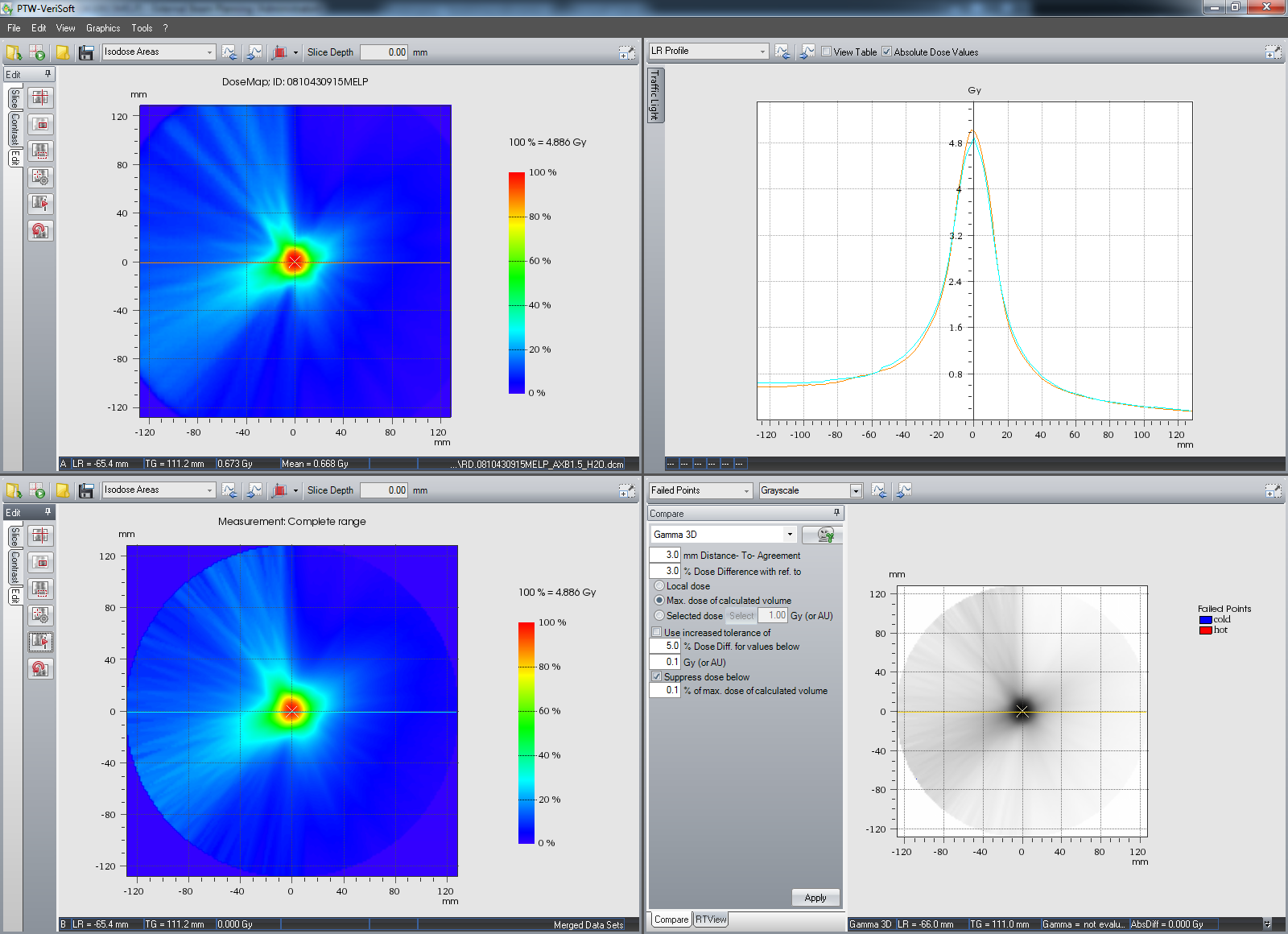
All but 40 evaluated voxels passed the 3G3 test:
The same merged measurement analyzed with 2G2 reveals that dose levels in the high dose region (> 85%) fail. One reason could be that the chambers are simply too large for such small targets. But there could also be other reasons.
If the user feels the need to squeeze out some tenth of a percent, it is worth trying whether "automatic alignment" of the two 3D matrices is able to improve it a little.
If once can live with the fact that 3G3 is passed but 2G2 is not, one can conclude that OCTAVIUS 4D 1500 can be used to verify even very small fields.
How would the result for 2G2 would have looked like without merging two measurements? The result substanciates the suspicion that spatial resolution is a key factor here.
Example 2 - Large Fields
Example 2 is a treatment of anal cancer, including lymph nodes. The plan uses the 10X flattened beam. Sometimes (like here) we have to add a third VMAT arc to get the desired target coverage, because the HD120 MLC has a rather limited maximum field size:
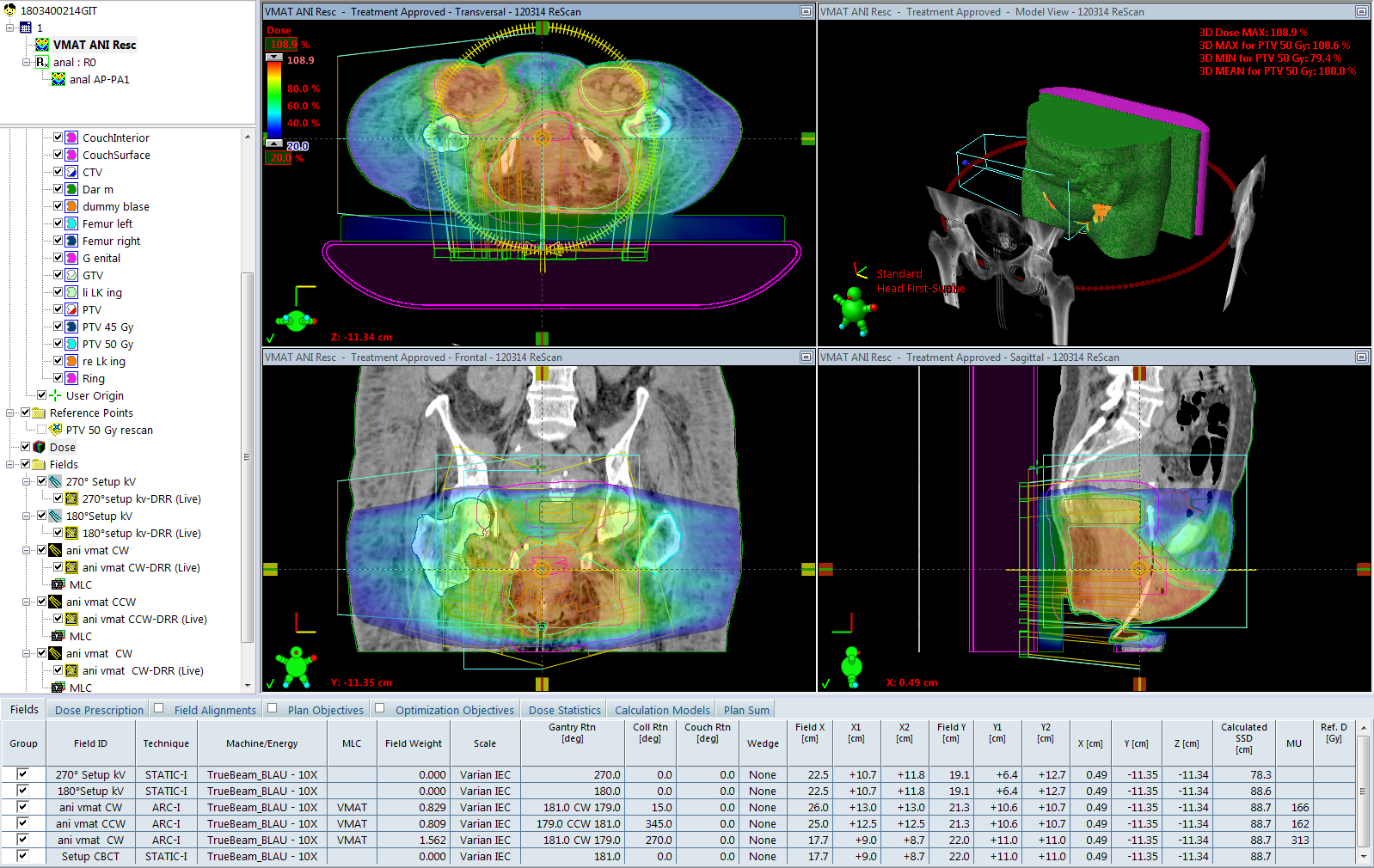
A large treated volume in the patient also means a large irradiated volume in the phantom.
Merging is not necessary to achieve a good verification result (2G2):
The volume analysis for 2G2:
The system has no problem with fields which irradiate the full volume of the Standard top.
A Remark on Grid Size
In Eclipse, the standard grid size for both AAA and AXB is 2.5 mm. For small targets (SRS etc.) we somtimes use smaller grids. Regarding the agreement between TPS and merged VeriSoft datasets, a higher resolution is not always "better".
In the following example, first the same measurement will be compared with two different AXB calculations.
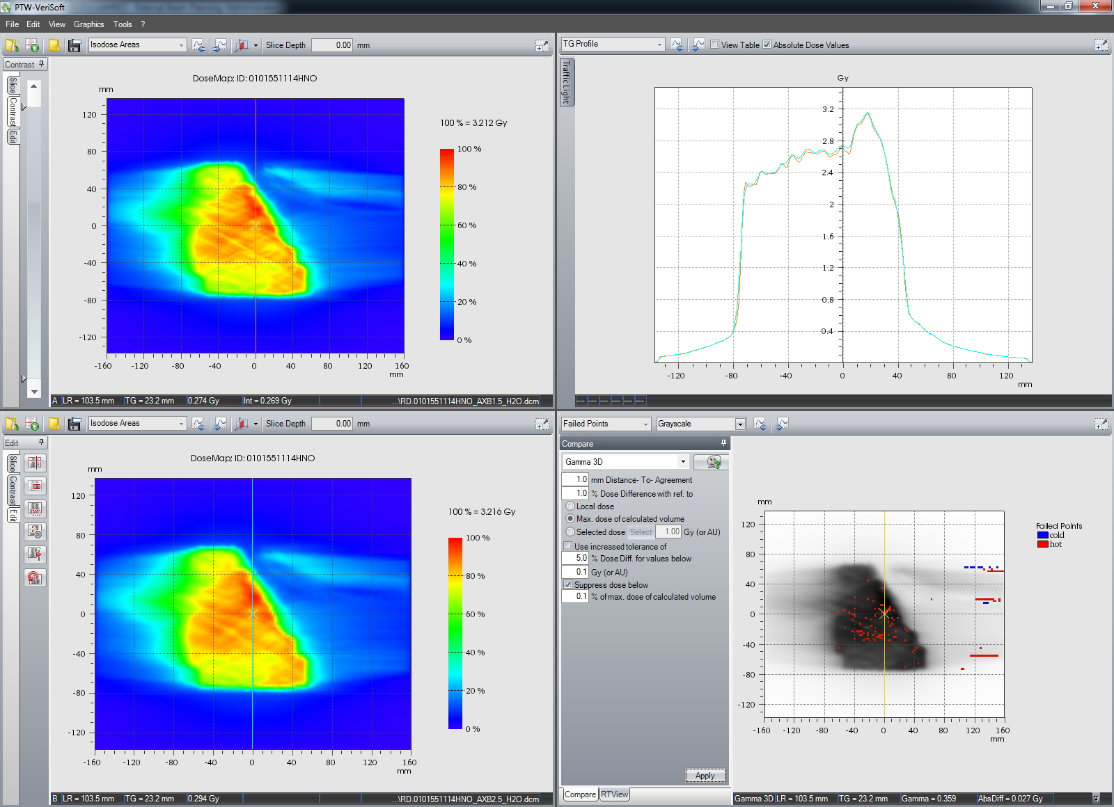
If AXB is set to a grid size of 1.5 mm, agreement (2G2) is worse,
than when the same plan is calculated with 2.5 mm grid1:
Keep in mind that the detector resolution is less than 2.5 mm, even in merged datasets.
We want to account for that in the next step.
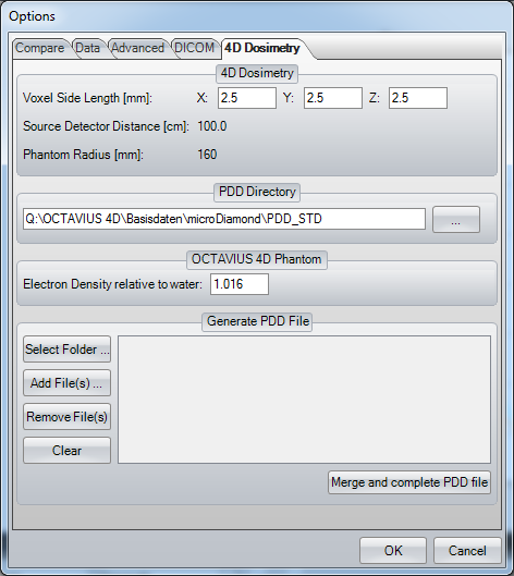
Now we keep matrix A, but repeat the reconstruction after we have changed the voxel size in VeriSoft from the previous value 1.5 x 1.5 x 1.5 mm to the new value 2.5 x 2.5 x 2.5 mm:

Again an improvement of the result! This confirms, at least for the example shown, the recommendation of PTW that the reconstruction voxel size and the calculation grid size should match. And it reduces calculation times, if unnecessarily small grids (either in the TPS or in VeriSoft) are avoided!
Notes
1A direct comparison of the two AXB dose cubes with 1.5 mm (matrix A) and 2.5 mm grid (matrix B) is also instructive. The gamma criterium was 1% global, 1 mm (1G1). There are even some voxels which fail the 2G2 test.