When an ideal (rectangular) fluence profile is going through a physical device like the DAVID chamber, the measured profile will be broadened ("blurred") due to the lateral transport of secondary electrons inside the chamber's windows and air volume. Even when the wires are perfectly aligned with the associated leaf pairs, they are not physically isolated from each other. When a single wire is hit by a small strip of radiation, some radiation will also be detected by the neighboring wires, and even by the wires at greater lateral distance. This phenomenon is described by the lateral response function (LRF) of the wire.
The following image shows the response of channel 15 to a 1 cm wide strip of 15 MV radiation from our Clinac (80-leaf MLC), measured with DAVID.

(static image, click to enlarge)
If there were no cross-talk, only channel 15 would detect fluence.
The goal of the deconvolution algorithm is to correct for this lateral response, and to reconstruct the original "sharp" fluence profile out of the measured "blurred" signal distribution.
Convolution/Deconvolution Demonstration with MATLAB
The convolution/deconvolution principle can be easily demonstrated with MATLAB (Release 2011b).
First we assume an ideal rectangular fluence profile, 10 cm wide, which is centered in DAVID's field-of-view. For the lateral response function of channel u (u = 1, ..., 40) we us a simple Gaussian,
![]()
where u is used to shift the Gaussian to the correct location. It is assumed that the LRF is the same for all leaf pairs (we will see later that this is not always the case). The factor in front of the exponential term is needed for normalization.
The parameter sigma controls the degree of "blurring". In the following animation, the rectangular profile is convolved with LRFs of increasing sigma (0 to 2):
(animated GIF, looping forever)
The higher the value of sigma, the higher the blurring. The effect is well known from scanning small fields in the water phantom with large-volume ionization chambers.
Let's choose sigma = 1. The measured signal will look like this:
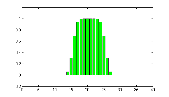
(static image)
How can we restore the original (perfectly rectangular) fluence from this measurement?
The Deconvolution Algorithm
The paper of Looe et al describes a simple iterative deconvolution method which "has been studied and used intensively, especially in the fields of spectroscopy and astrophysics for de-blurring measurement results, hence increasing their resolution."
If we call the (unknown) ideal rectangular fluence profile P(x) and the convolved measured signal profile S(x), we can write

for the convolution. The sum runs over the 40 detection wires, and also x is a discrete variable running from 1 to 40. The fluence profile P(x) can then be calculated in an iterative deconvolution loop with the help of two simple equations:
![]()
and

The first equation should converge towards the "limiting function" P(x), the second is the calculated signal in iteration step n.
The loop starts with the initial assignment
![]()
This method has been implemented in David 2 software. The complete algorithm contains a termination criterion which is not described here, but which is necessary due to statistical noise in the measured signal.
The algorithm is fast enough so that measurements can be processed in real-time. To make this point clear: it is so fast that the user does not even notice that the real-time display during the measurement is already deconvoluted. This is in contrast to the three idealistic animations which will be shown next, where every single iteration will be plotted.
In our example, let's assume that we don't remember the sigma value we have chosen. We will use try-and-error, select three different sigma values, and check the deconvolution outcome.
First we try sigma = 0.95. The following slowed-down animations show every single iteration in the iteration loop:

(animated GIF, looping forever)
With every frame, the iteration index n is incremented by one. The result is already quite good, but the profile could be a little sharper. Now we try sigma = 1.00:

(animated GIF, looping forever)
After several iterations, the exact rectangular profile is perfectly restored!
One more try with sigma = 1.05:

(animated GIF, looping forever)
The edges of the profile are clearly too sharp. Even worse: the iterative process is not converging. This is an indicator that the selected sigma is too large.
Of course we know that sigma = 1 is the correct answer, because we knew the primary fluence profile. In the real world (using David), the primary fluence profile is unknown, but the lateral response function (described with the single parameter sigma in our oversimplified model) can be determined experimentally for each leaf pair. This is described next.