2D-Calibration of the Enhanced Leaf Model - Part I
Introduction
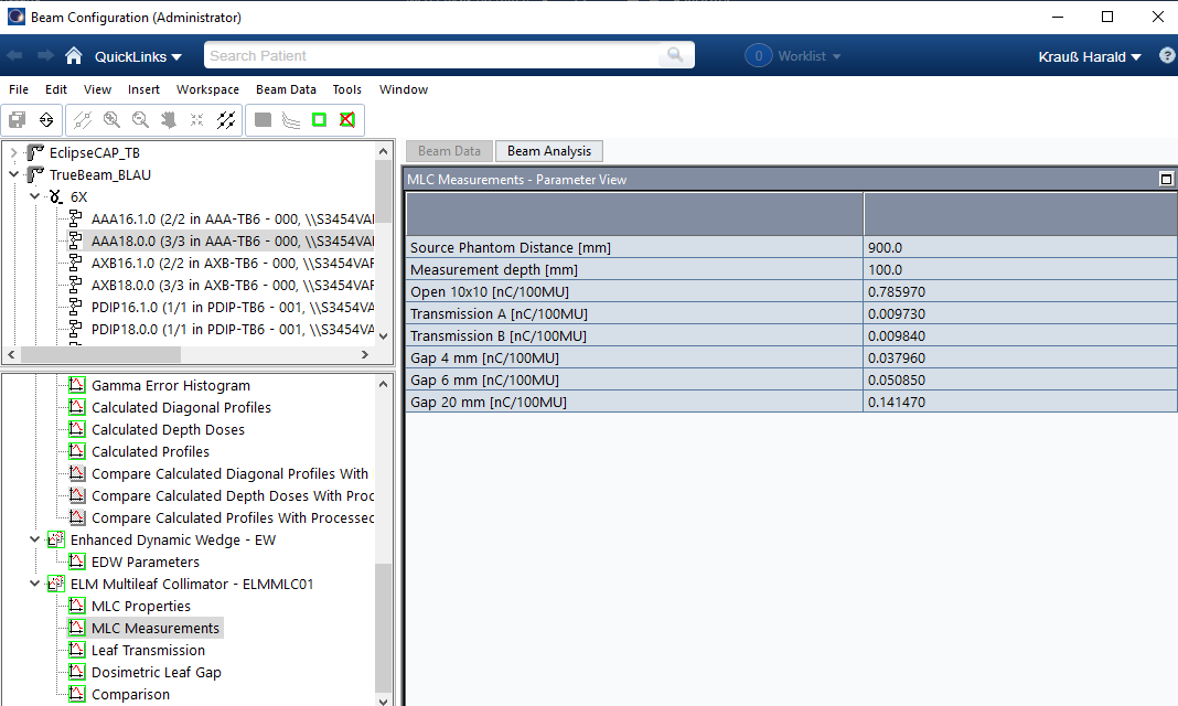
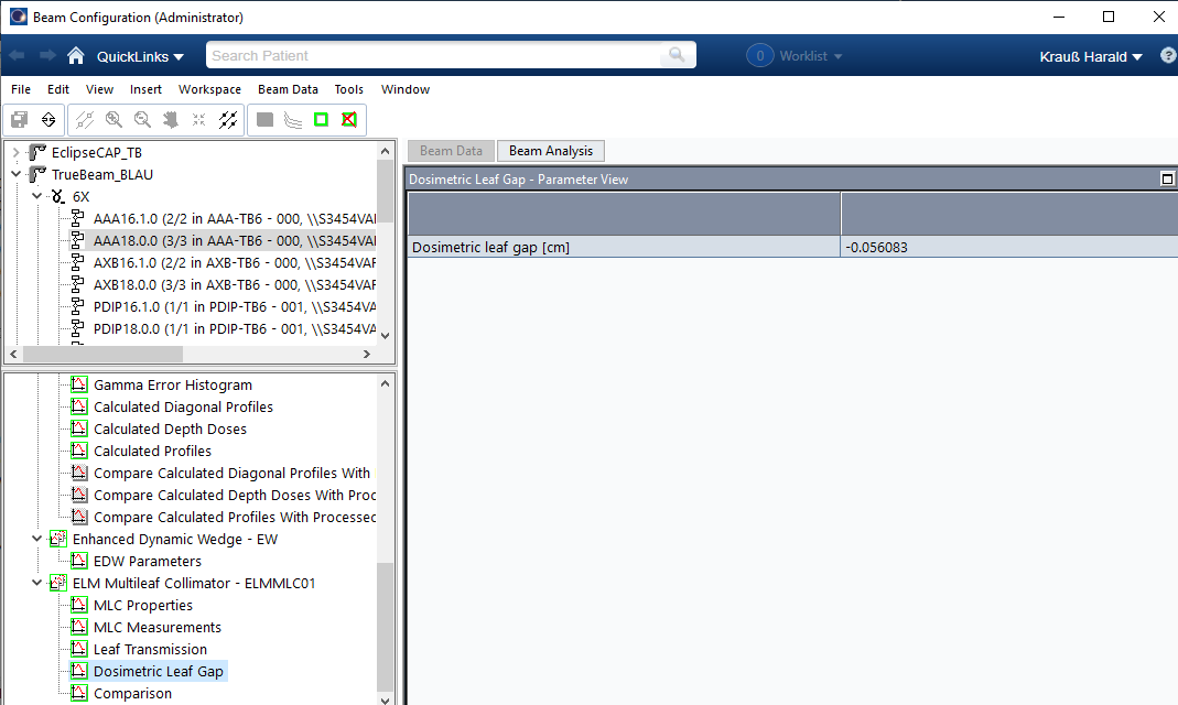
The dosimetric configuration of the Enhanced Leaf Model (ELM), which was described recently, involves one crucial step: the measurement of dose values for a series of six calibration fields (Open, TrA, TrB, Gap4, Gap6, Gap20). The measured values are used by the optimization routine in Beam Configuration to calculate the dosimetric ELM parameters average leaf transmission (Tr) and dosimetric leaf gap (DLG).
Varian's recommendation is to use "a larger volume ionization chamber, such as Farmer" for the measurement. This is where we hook in.
Robustness
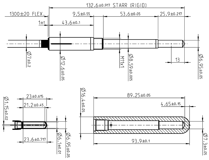
The sensitive volume of a Farmer chamber such as the PTW 30013 has a length of about 2 cm. This means that if the TrA or TrB field is loaded on the HD120 MLC, at isocenter distance the chamber will "sense" the intraleaf leakage of approximately ten leaves, plus nine interleaf leakages:
Will the transmission values measured in this way be representative?
We know from any 1D or 2D measurement under a closed MLC, that the interleaf leakage between neighboring leaves on the same bank is not constant. Some peaks are higher, some are lower.
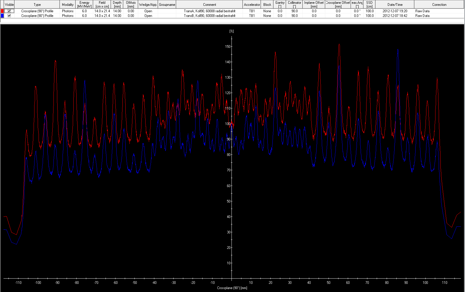
These profiles show 1D-scans under leaf bank A (red) and B (blue) for the HD120 MLC, measured in water with a resolution of 0.1 mm1. Both curves are normalized to 100% at CAX. TrA (red) seems higher on the average, but this is beause local transmission at CAX is relatively low.
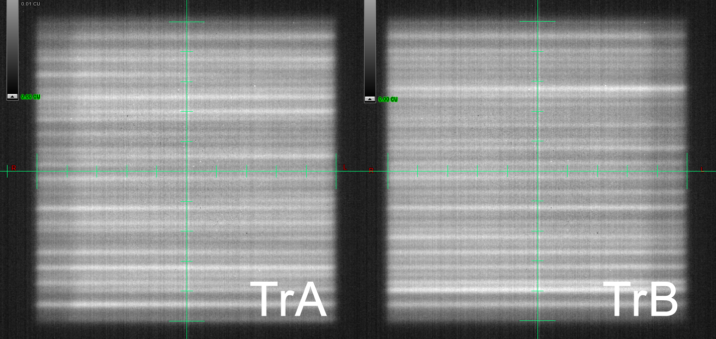
The next image shows the 6FFF integrated images of the TrA and TrB calibration fields during acquisition on TrueBeam BLAU (full screenshots here and here). Note the irregular pattern of darker and lighter stripes, signifying lower and higher interleaf leakage, respectively:
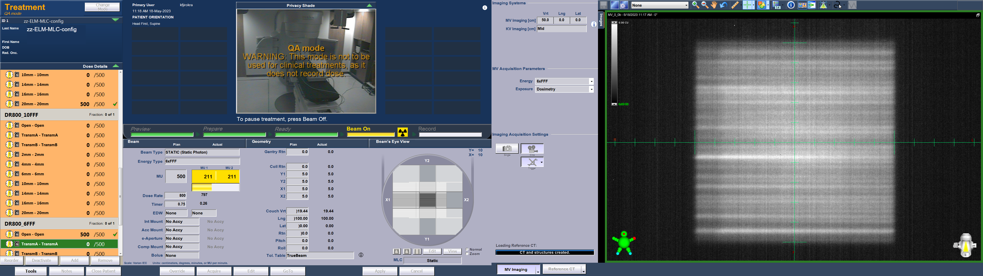
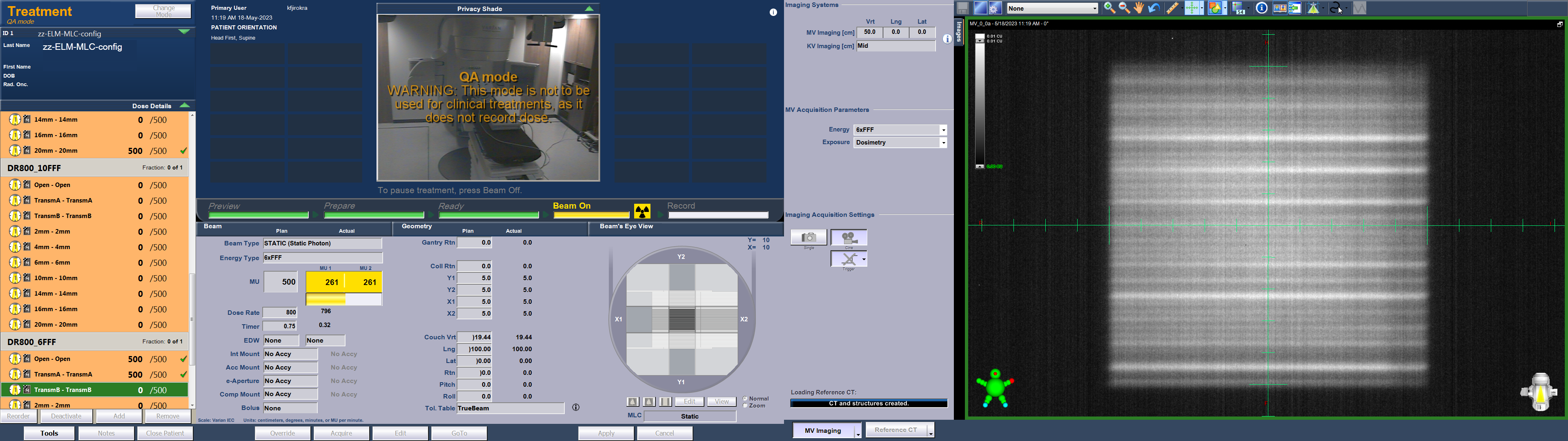
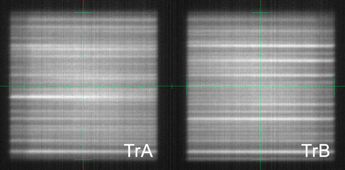
If darker of lighter stripes are more frequent in the central area, the Farmer's sampling size might not be sufficient, leading to an under- or overestimation of Tr. A similar image from TrueBeam GRÜN (6X) is shown here.
When comparing different machines, it is also fair to assume that there will be small differences regarding MLC dosimetry.
The lack of perfection may also have an effect on Tr values measured at different gantry angles. It is not unconceivable that under the influence of gravity, the interleaf leakage may change.
Clinical VMAT or IMRT treatments are performed at all possible Gantry angles, so we look for a "robust" dosimetric modelling, which will be truly representative for any clinical situation.
Instead of relying on the "intrinsic averaging" of an ionization chamber, more robust measurement results can possibly be achieved by using 2D instead of single point measurements. With better statistics and wisely chosen sampling areas, averaging over these regions of interest (ROI) may give more representative values for the ELM dosimetry configuration.
Materials and Methods
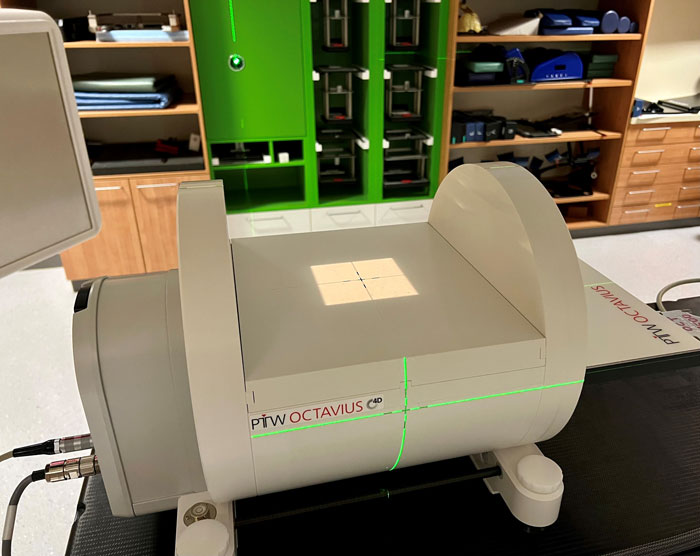
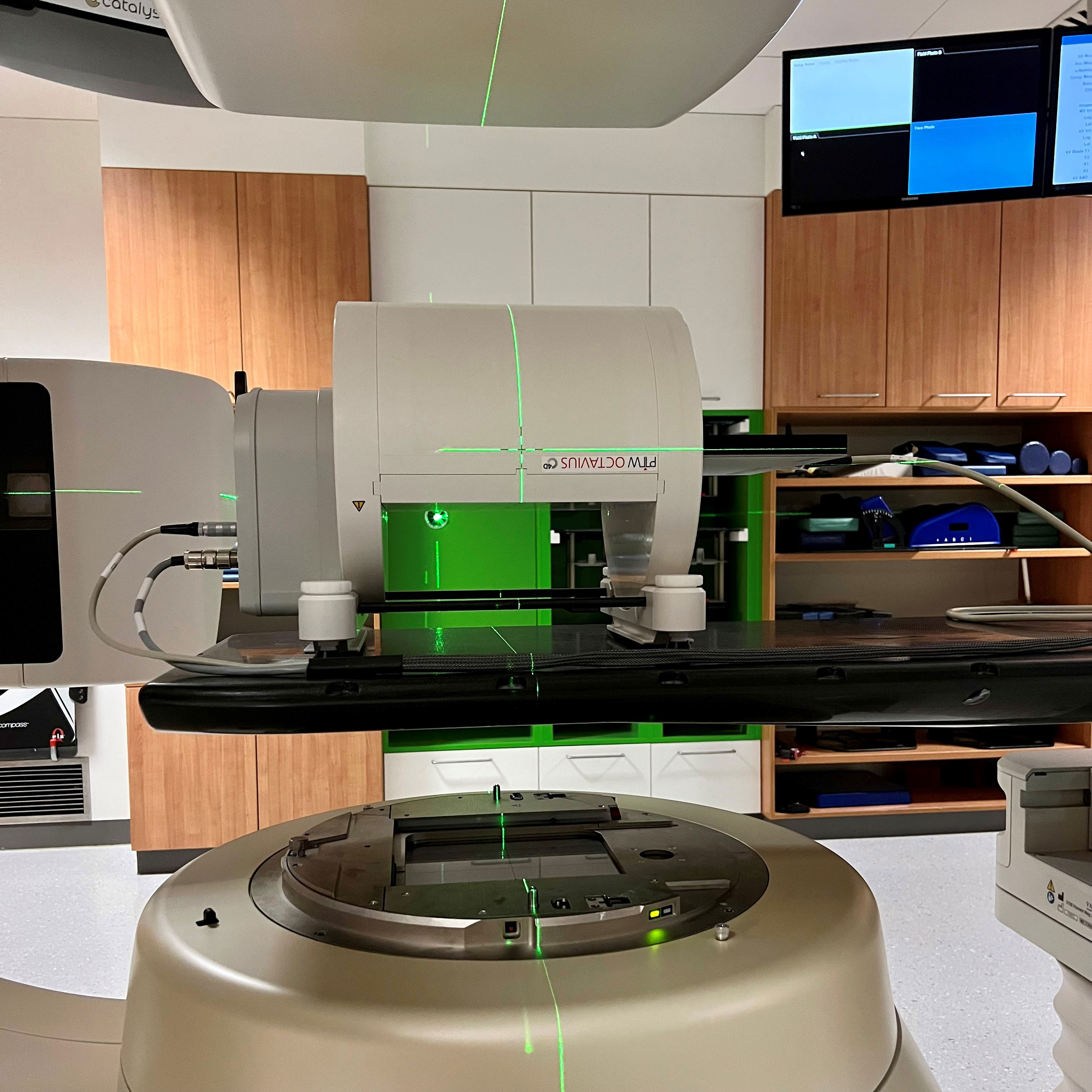
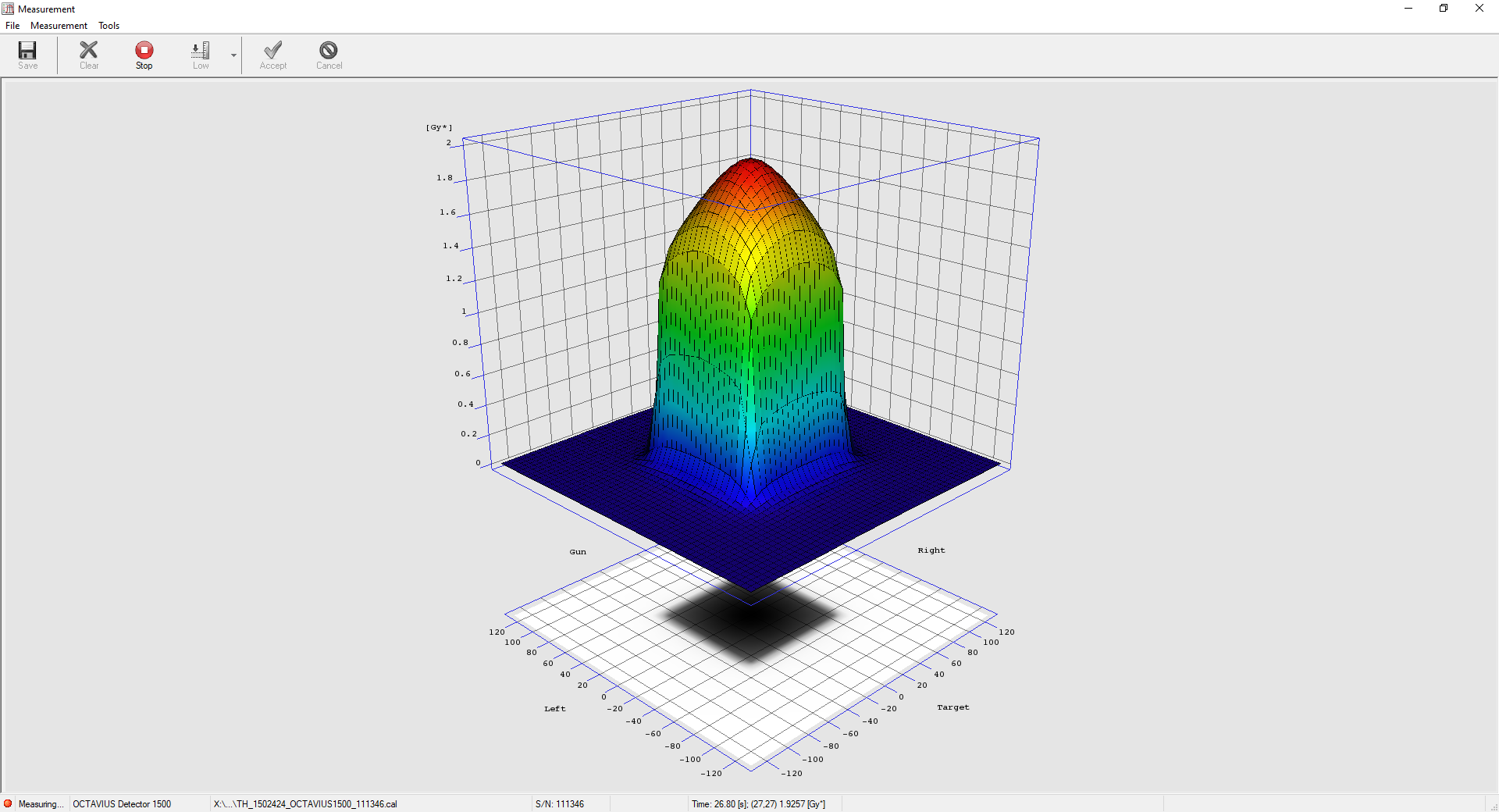
The OCTAVIUS detector 1500 is used to measure2 the six calibration fields. The Rotation Unit has a flat top designed for Linac QA. Although the measuring depth of 5 cm does not strictly follow the Varian recommendation of 10 cm, we will use this setup3 for convenience:
As described elsewhere, by merging two consecutive, longitudinally shifted measurements, the field coverage can be doubled4. We use this feature throughout the study.
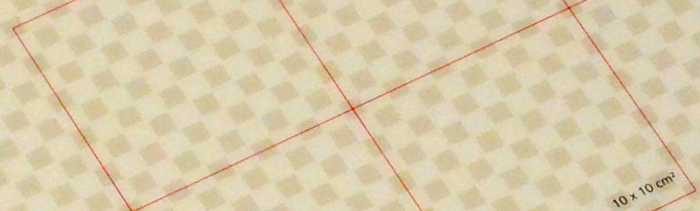
(Surface of OCTAVIUS Detector 1500. The darker squares mark the locations of the ionization chambers.)
For each of the six fields, a representative ROI is chosen, and the values inside the ROI averaged to give a single value. Depending on the ROI's size (see below), this averaging is either over 169 or 143 values per field. Evaluations are done with PTW VeriSoft 8.1 and Excel.
Transmission Measurements
The ROI size for the Tr fields must be carefully chosen. The ELM model requires that Tr is measured under the screw cutout area of the leaves, which for the TrA and TrB fields is certainly the case at CAX. But when a larger area is used for averaging, care must be taken so that the ROI does not extend into the full leaf area.
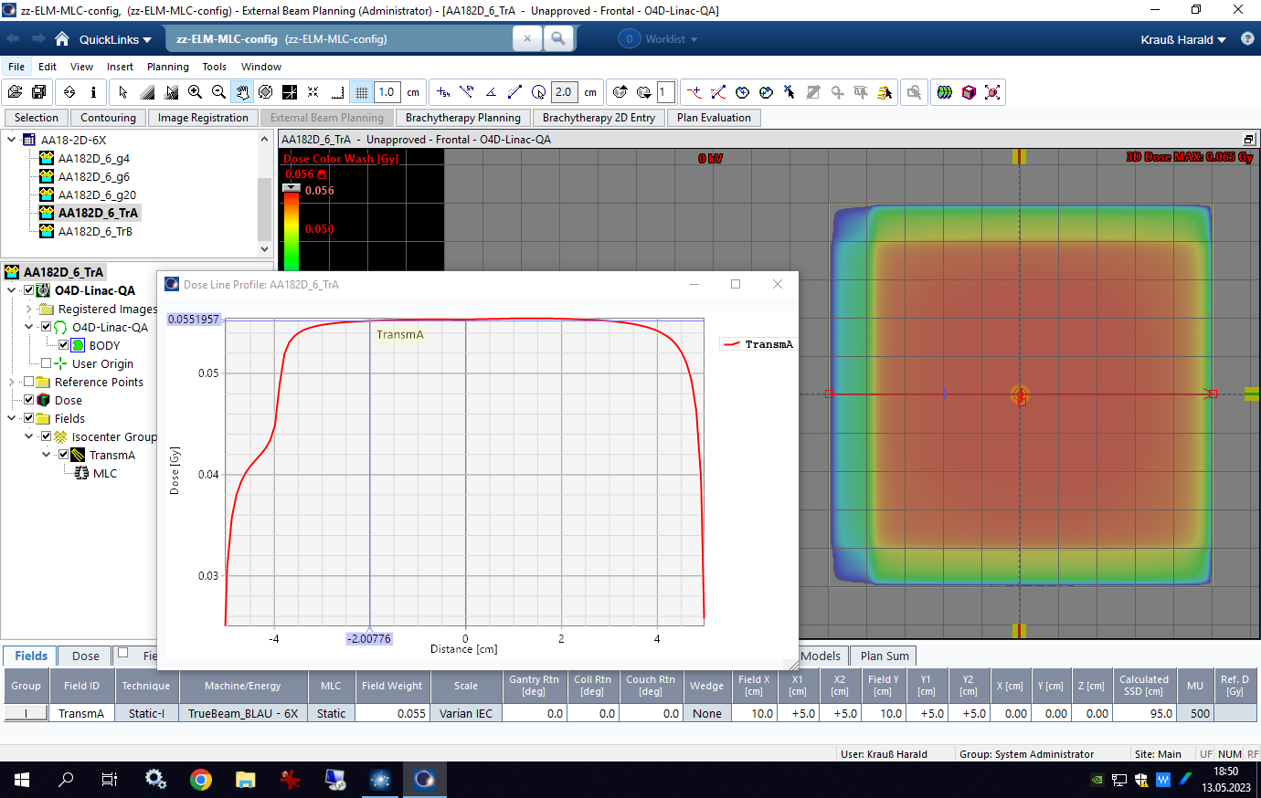
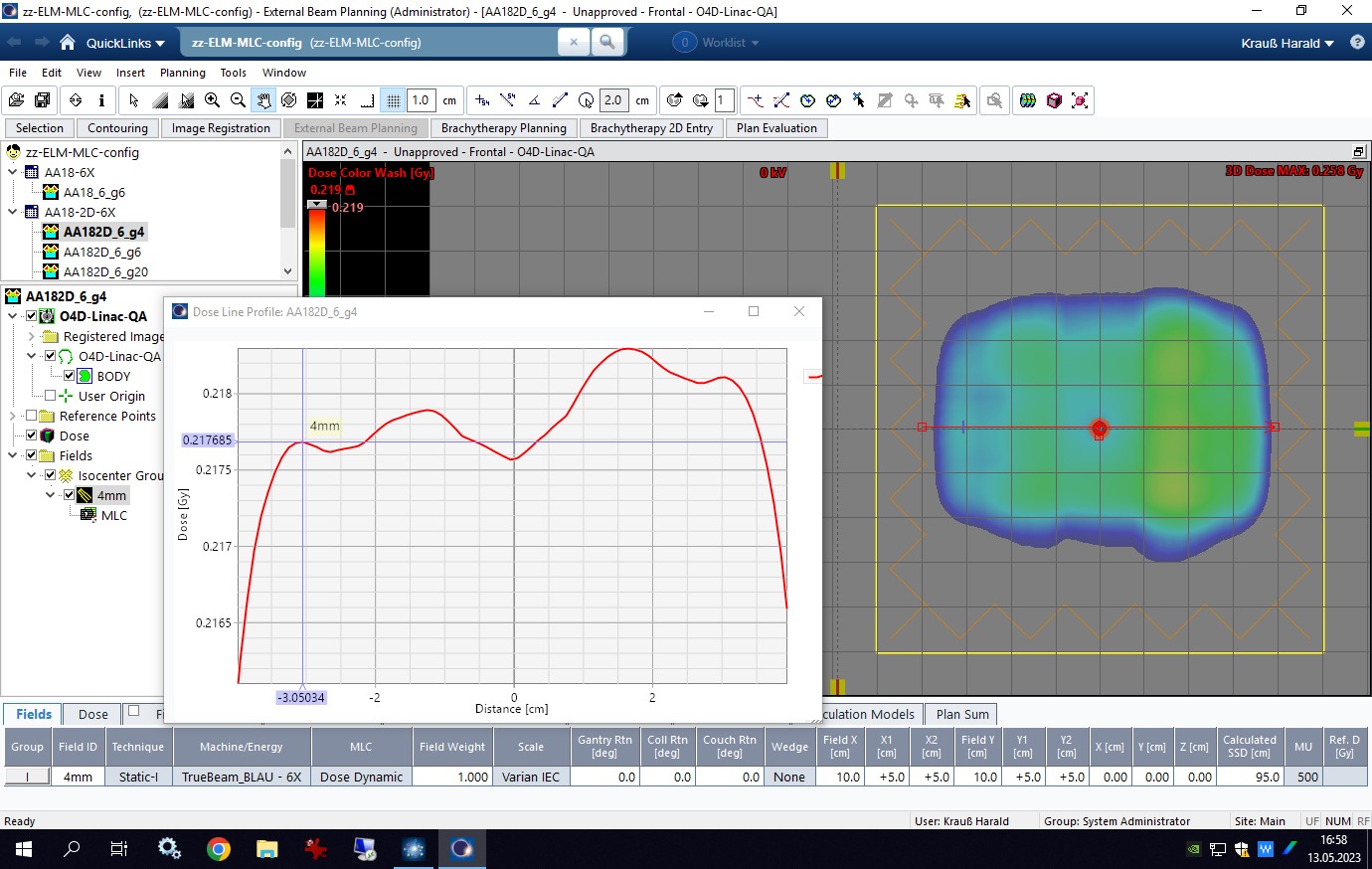
We can simulate this in Eclipse using a preliminary model. In 5 cm depth (6 MV field), the TrA profile is very constant up to 3 cm off axis in X2, Y1 and Y2 directions. In X1 direction (left edge of the field), the profile breaks in earlier, because the screw cutout area ends and the full leaf part begins. Here we stop the sampling at 2 cm off axis (blue cursor):
For TrB, the situation is mirrored. For the averaging, the area chosen will be 50 mm wide (asymmetric) and 60 mm long. With the 2D array's chamber spacing of 5 mm, this corresponds to 11 x 13 = 143 sampling points.
Gap Measurements
In the direction of leaf movement, an area which is much wider than the width of the Farmer's sensitive volume (6.1 mm) can be used for sampling, because the sweeping gap spans the full 10 cm field width.
But are really all sampling positions in the field equal in the sense that they see the same mixture of gap, full leaf transmission and cutout transmission?
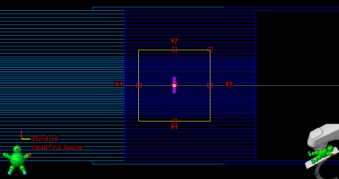
The following image shows Gap4, the sweeping 4 mm wide gap field, in BEV shortly after beginning. All leaves move at constant speed from left to right while the beam is on. The right leaves (bank A) are retracting. If we focus on the measurement point in the center of the field, the chamber is just starting to "see" the transmission signal going down a little, because the retracting leaf ends to expose the screw cutout area and starts to project the full material cross section, which begins 3 cm behind the leaf tip.
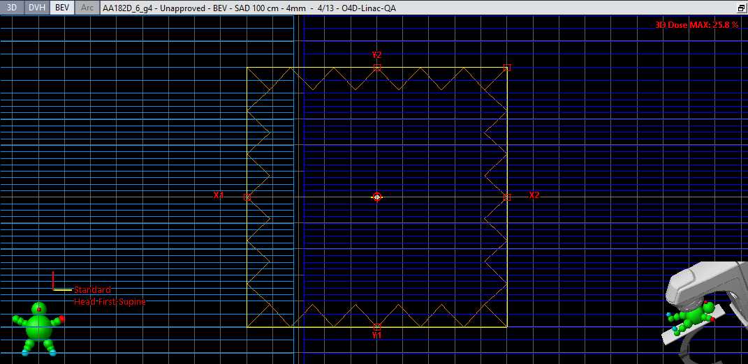
Strictly speaking, only those sampling positions inside the field which see the same mixture of gap, full leaf transmission and cutout transmission can be considered as dosimetrically "equal". For the field shown, this area is 6 cm wide (if we assume that the screw cutout transmissions of bank A and B are identical).
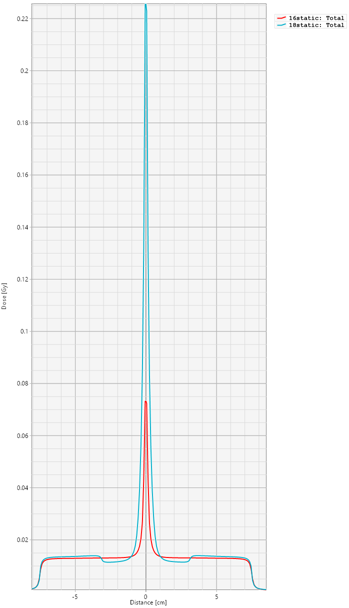
However, we don't think that the small difference between full leaf transmission and screw cutout transmission really matters, because they are both much smaller than the dose contribution from the sweeping gap, by orders of magnitude. Consider the height of the blue (ELM) profile (which is for a fully closed leaf pair, not for a gap!).
The calculated Gap4 dose (AAA calculation grid size: 1 mm) supports this assumption. Apart from the arkward asymmetric shape of the profile in 5 cm depth (another story), the range from -3 cm to +3 cm looks fairly constant.
What about inplane? The outermost 1 cm on the Y1 and Y2 side must be excluded from sampling in any case, because they are under the 5 mm thick leaves. This reduces the theoretical maximum sampling length to 8 cm. From the calculated dose distribution in our preliminary model, one can see that inplane dose is again fairly constant over the central 6 cm.
For averaging of the gap fields, we therefore choose a ROI of 60 x 60 mm5, corresponding to 13 x 13 = 169 sampling points instead of a single (Farmer) value. The same ROI is used for the Open calibration field, which serves as reference for the other five calibration fields.
Right after averaging and configuring the ELM dosimetry, the model can be validated using the same fields (which will be covered in Part II). This is the beauty of the 2D calibration: the 2D-calibrated ELM should be able to model the measured dose distributions of both the TrA and TrB fields (on average), plus the three gap fields Gap4, Gap6 and Gap20.
Gantry Dependence
So far, we operated at Gantry 0° only. To check for gravitational influence, measurements at the four major gantry angles are carried out for 6 MV. This way, we let the leaves sweep up against gravity (Gantry 270°) and down (Gantry 90°). For each setup, a full set of six calibration fields is measured, and compared to the reference at Gantry 0°.
At Gantry 180°, the beam passes the PerfectPitch couchtop. The effect of the carbon couchtop on Tr and Gap values should be small, because measured values are always relative to the Open field, which passes the couch as well.
All fields (500 MU) are delivered at a dose rate of 600 MU/min (800 MU/min for 6FFF and 10FFF). To check the alignment on the phantom, this happens under the watchful eye of the DMI detector:
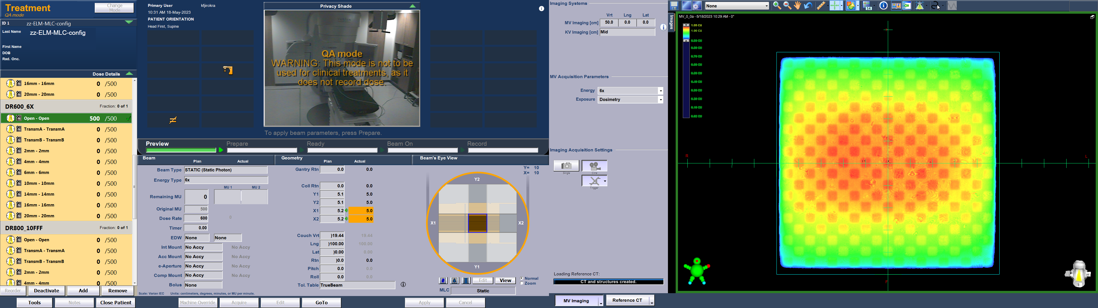
This animation shows the (slightly sped up) delivery of the 15X Gap4 field on the TrueBeam. The gap starts under the X1 jaw, so the very first frames show the typical TrA pattern (darker vertical band on the left):
Results
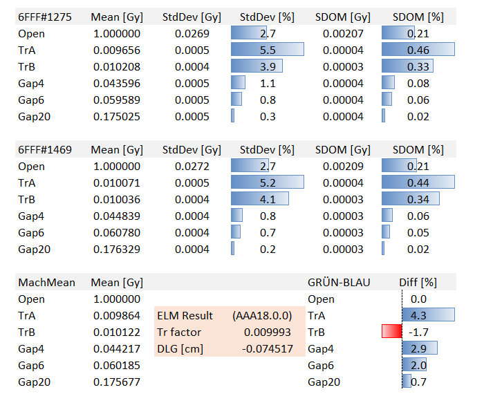
The following table reports the results for 6X, Gantry 0°, individually per machine (TrueBeam BLAU, #1275 and TrueBeam GRÜN, #1469) and as average over the two machines ("MachMean"). These values could be entered directly into Beam Configuration to configure ELM dosimetry. The box in pink shows the result of the optimization routine:
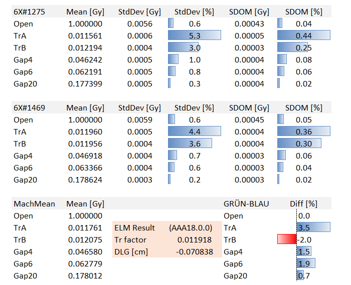
We normalized all measurements to the "Open" field because the configuration routine would do it anyway. The sample standard deviation StdDev for the ROIs and the standard deviation of the mean (SDOM) are both given in [Gy] and in [%]. The differences between the machines, e.g. 3.5% for TrA, seem rather large. However, this is a relative number. The absolute difference is 1.196% - 1.156% = 0.04%.
To exclude the influence of the profile shape on the statistical values, the statistics of the Tr and Gap fields was calculated as follows: for each location in the 2D matrix (chamber position), Tr and Gap values were divided by the respective "Open" field value first, and then the statistics was calculated. This way, the shape of the beam profile (especially for the FFF energies, but also for 15X) cancels out and does not influence StdDev and SDOM values.
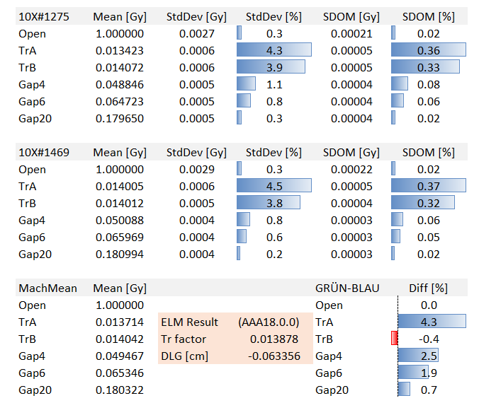
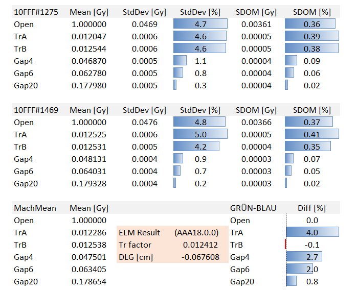
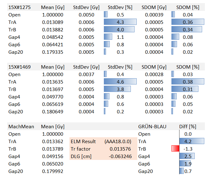
See also the results for the other energies (6FFF, 10X, 10FFF, 15X).
Gantry Dependence
The next table contains the results for the major Gantry angles on TrueBeam GRÜN and 6X, plus the Gantry mean values ("GMean"). Both the Tr and the Gap doses increase when the Gantry rotates down, with the largest values measured for Gantry 180°:
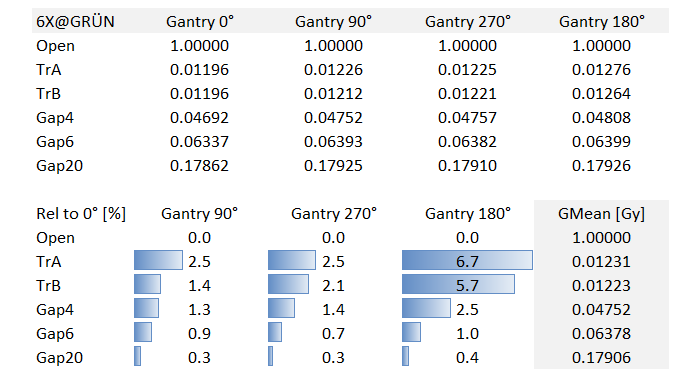
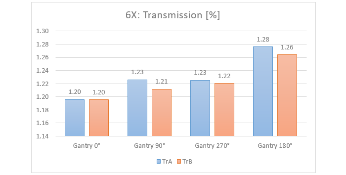
Transmission TrA for instance increases by 6.7% (1.276% instead of 1.196%). The Tr data put in a diagram:
ELM2D or ELM2DG?
Before the Eclipse calculation models can be configured, a decision has to be made whether Gantry dependence (the data from the last section) shall be included or not. On one hand, the knowledge that the values measured at Gantry 0° were the lowest of all should not be ignored. On the other hand, data was measured only for one energy, and only on one machine. And it is not fully clear what the outcome would be for collimators rotated to, say, 45°, or for intermediate Gantry angles6.
To get an idea of the impact, we quickly configure two AAA calculation models: one model (ELM2DG) uses data of all Gantry angles (on one machine), the other model (ELM2D) uses only the Gantry 0° data (averaged over two machines). Otherwise, the models are identical. From the optimization routine, we get the following ELM results:
- ELM2D: Tr = 0.011918, DLG = -0.070838
- ELM2DG: Tr = 0.012269, DLG = -0.063791
We then choose an arbitrary complex test pattern and compare the calculated doses (grid: 1mm). Upper left is the ELM2D calculation, lower left is ELM2DG which takes the Gantry measurements into account. In the Gamma analysis (1%/1mm), there are only very few, small areas where a difference can be spotted:
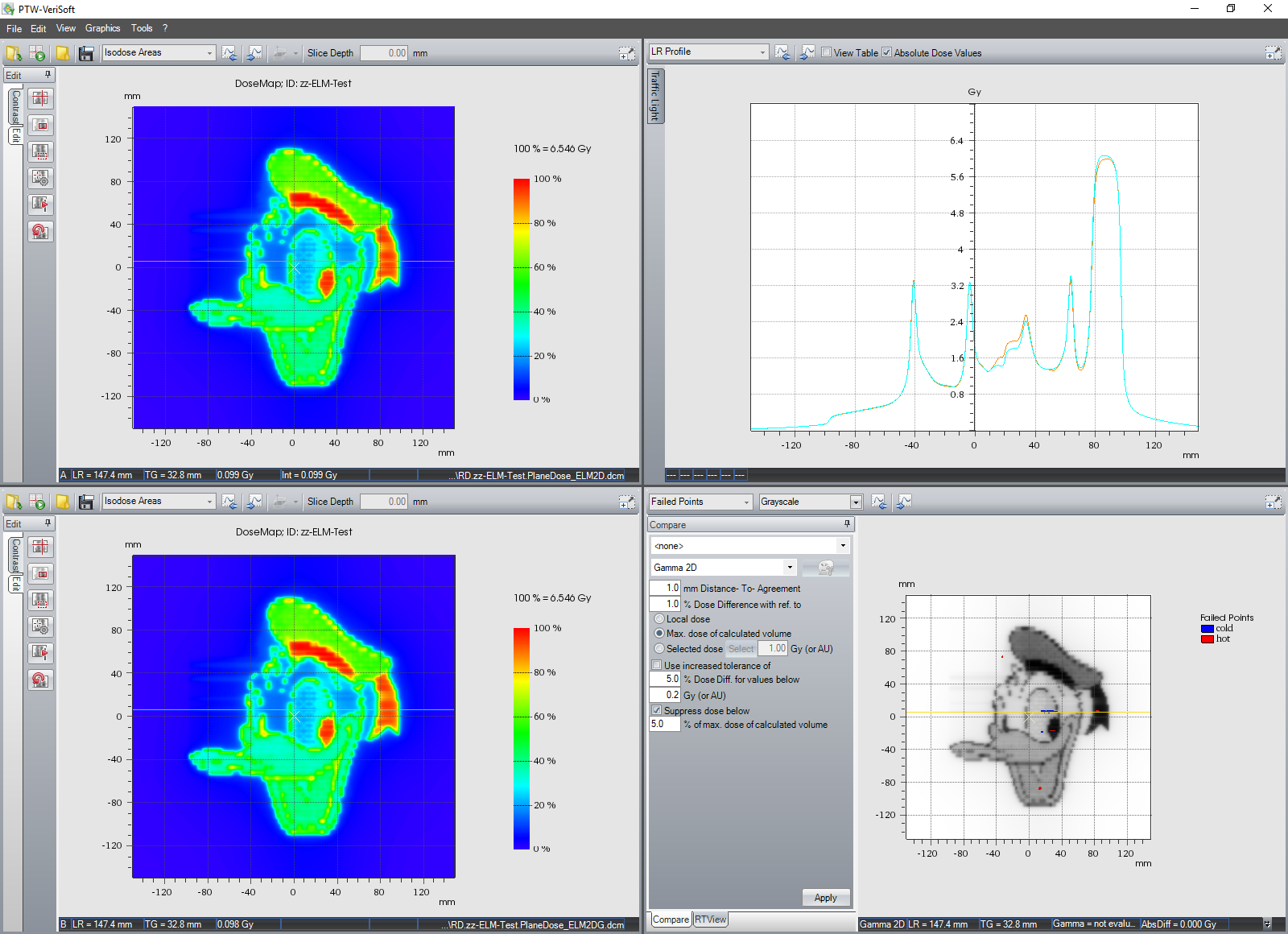
This quick check suggests that it should be OK to use data acquired at Gantry 0° only. If the calculations are nearly indistinguishable, there is no need to compare them with measurements.
Summary
It was demonstrated that for the ELM configuration it is possible to measure the required data with a 2D Array instead of a single ionization chamber. The acquisition is straightforward and offers some new possibilities.
Another article (Part II) will cover validation. After ELM dosimetry configuration has been performed, the Eclipse calculation models ideally should be able to reproduce measured 2D doses of the five calibration fields where an MLC is involved in a self-consistent way.
Measuring the six calibration fields for 5 photon energies on one machine at Gantry 0° took less than 2 hours (6 x 5 x 2 = 60 fields).
Notes
1 The PTW photon diode 60008 contains a semconductor chip which is only a few micrometers thick. Spatial resolution can be maximized by irradiating the detector radially, i.e., from the side.
2 Each field is measured multiple times without mentioning.
3 We assume that the results will not differ significantly if 5 cm are used instead of 10 cm.
4 The 5 mm longitudinal couch shift can easily be performed remotely from the control room.
5 The ROI size 60 x 60 mm refers to the chamber centers. The actual sampling area is larger (65 x 65 mm).
6 With the Rotation Unit and considering the (static) transmission fields, it would be easy to measure dynamically (while the Gantry rotates), because the Array rotates with the Gantry. For the Gap fields however, this is more tricky. And which collimator angle to choose?