2D-Calibration of the Enhanced Leaf Model - Part II
Validation
The data measured with the OCTAVIUS Detector 1500 for the six calibration fields was used to configure the Eclipse calculation models. Because small dosimetric differences exist between the two machines, we used the "MachMean" averaged data as described in Part I.
As a consequence, there will always be a certain disagreement between calculation and measurement, since the calculation is based on an "average machine" that does not really exist.
For instance, the 10FFF transmission TrA on GRÜN is about 4% higher than on BLAU. This means that when the 10FFF Gap4 field is calculated in Eclipse and compared to the measurements that were used to configure ELM dosimetry, calculated dose is a little too high compared to measurement on BLAU, and a little too low when compared to GRÜN.
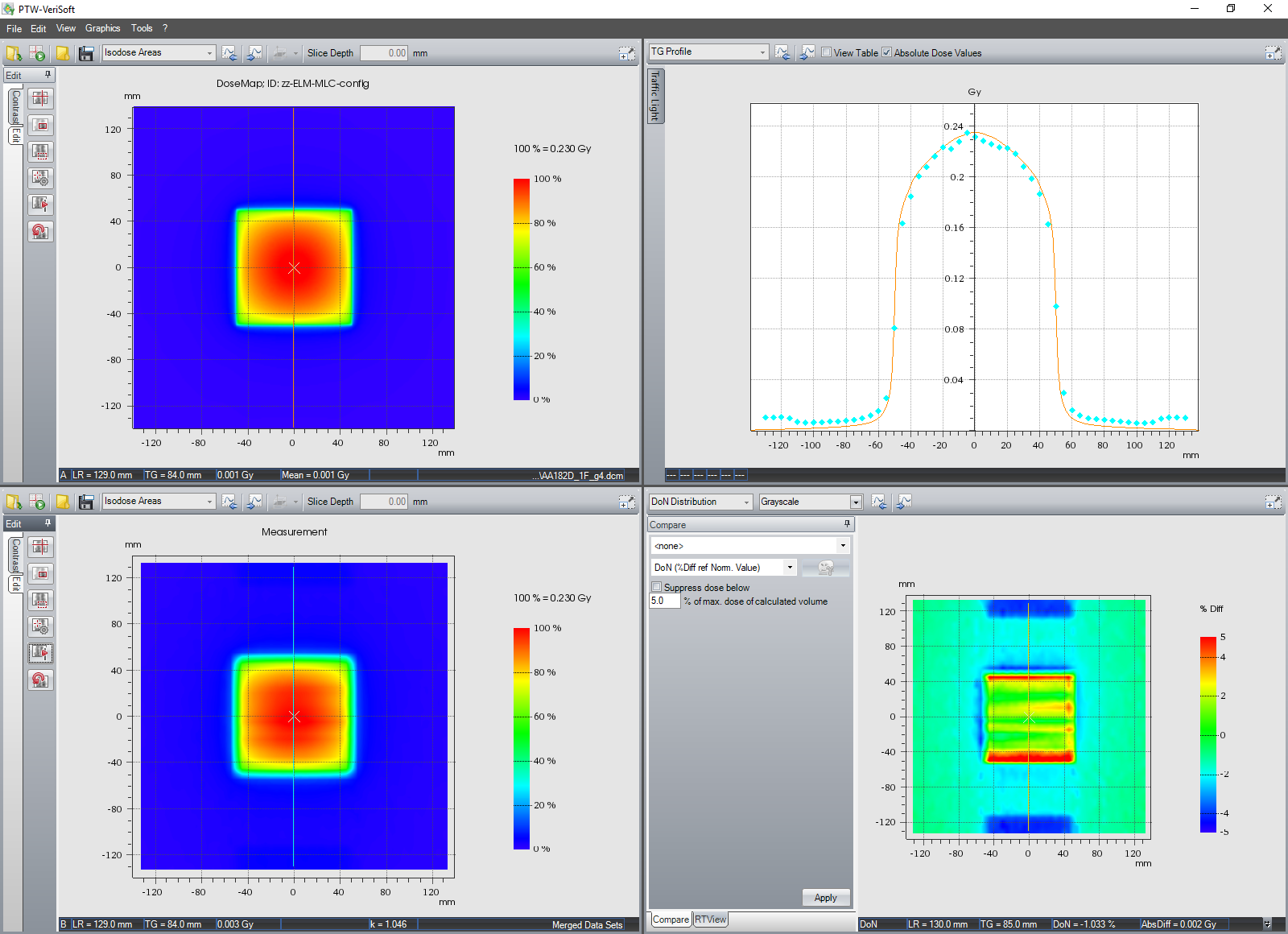
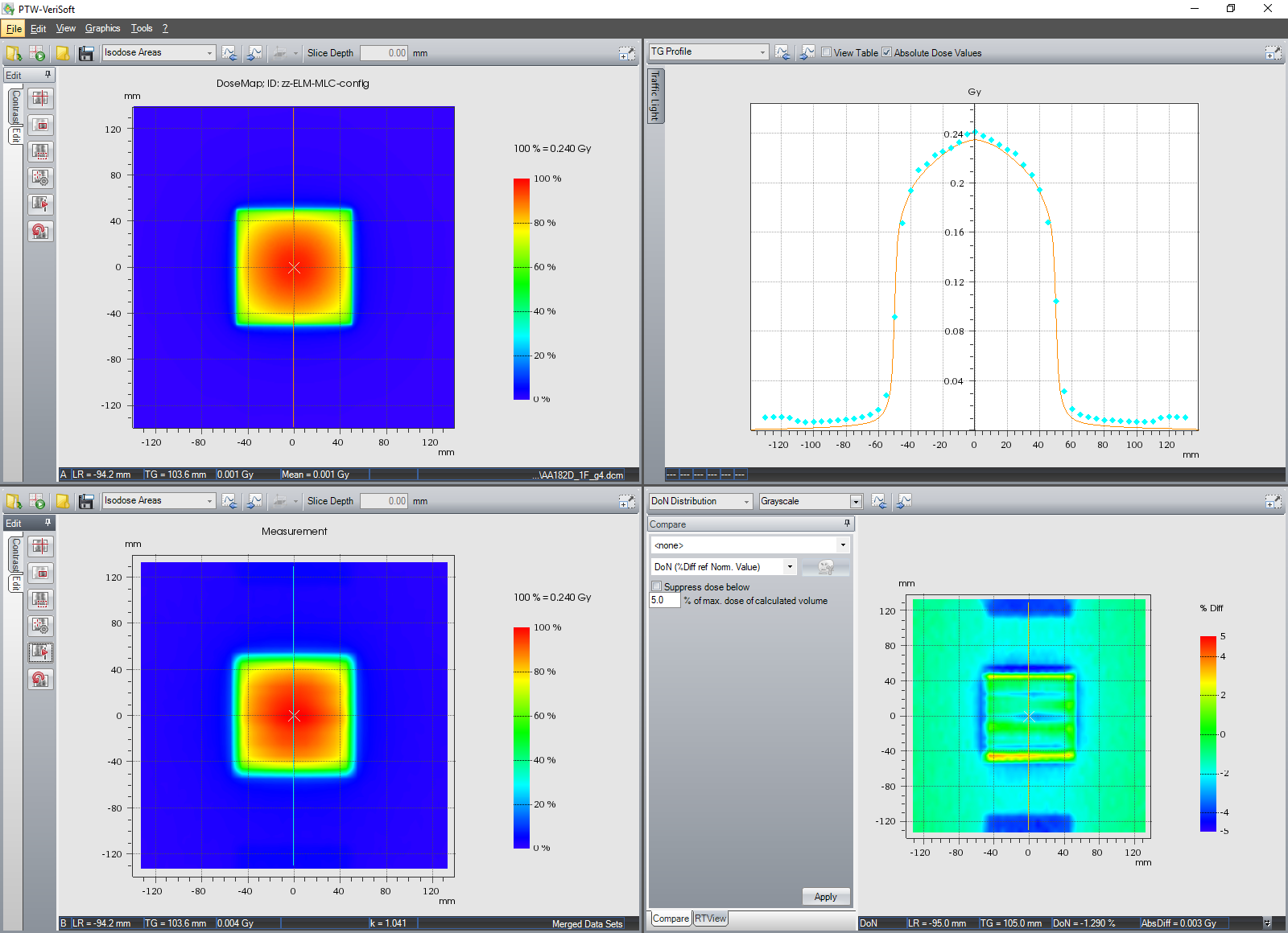
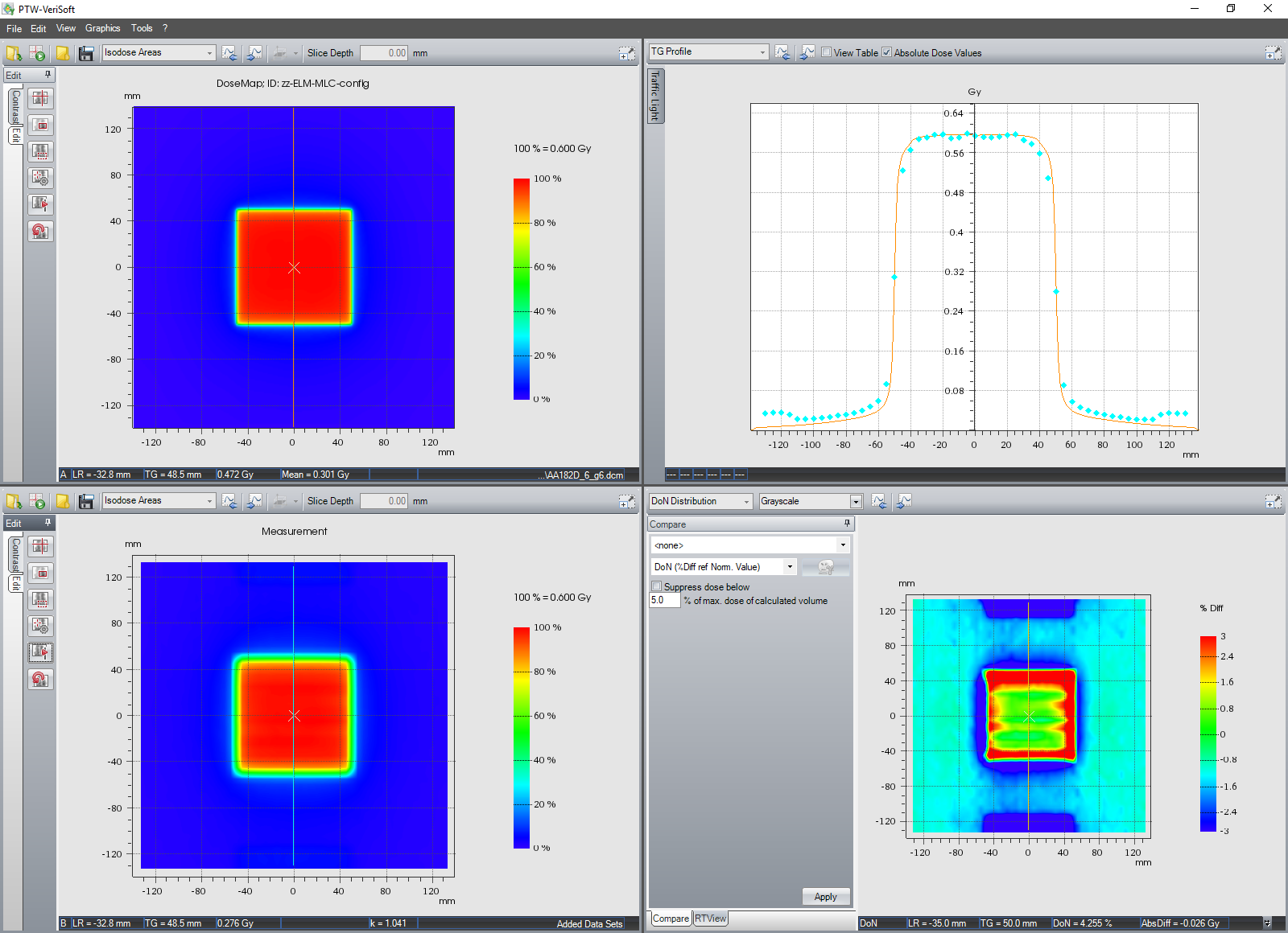
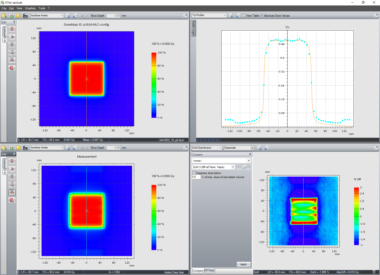
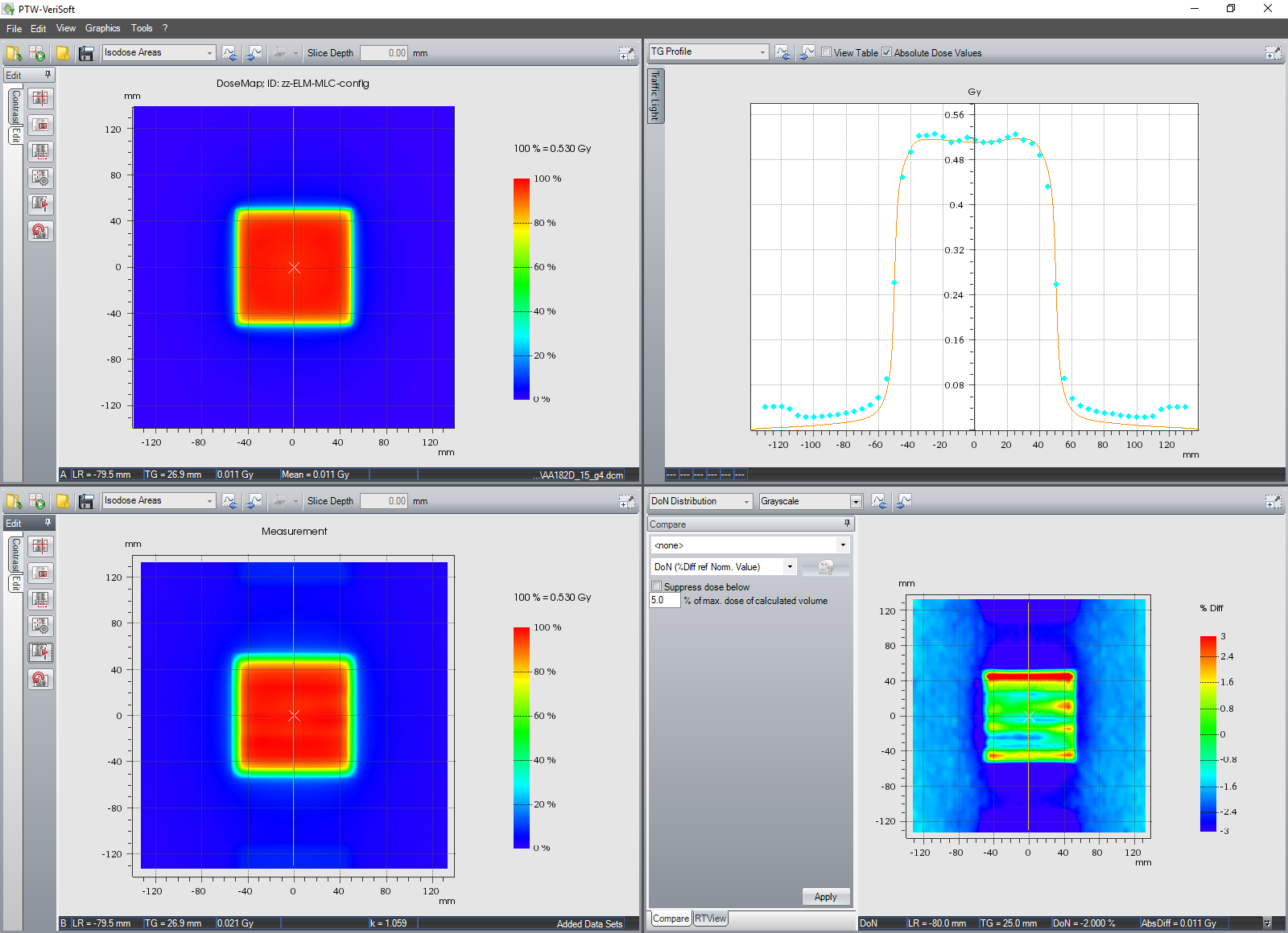
One way to solve this - although the method is rather impractical for clinical plan validations - is to measure the same field on both machines, add the 2D doses, and compare the result to the doubled Eclipse dose. For the Validation fields we can do this, because they were measured on both machines anyway. Here the inplane profile through the mentioned Gap4 field, after summing as described. Matrix A is twice the Eclipse dose, B is the measured sum BLAU + GRÜN. Agreement is very good:
To complete the validation, we calculated the five calibration fields TrA, TrB, Gap4, Gap6 and Gap20 in Eclipse, and compared the 2D dose distributions to both measurements (BLAU and GRÜN). This gives 50 comparisons for the five photon energies.
Validation of Tramsmission Fields
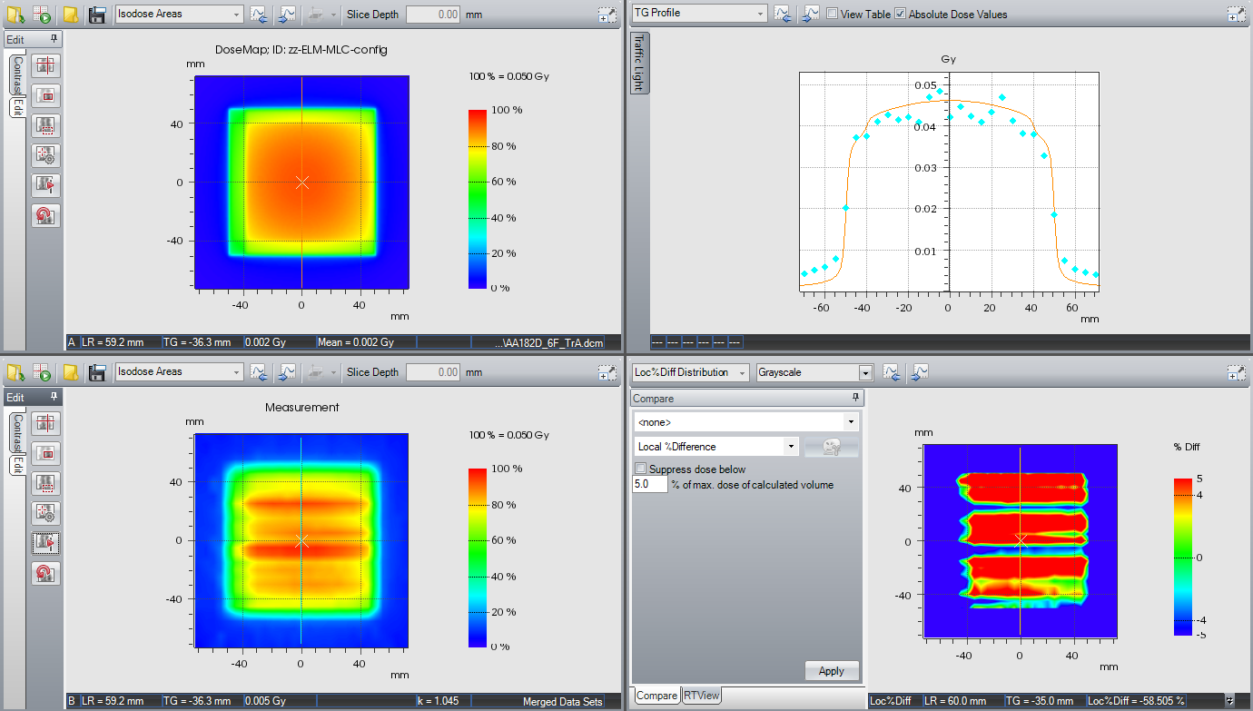
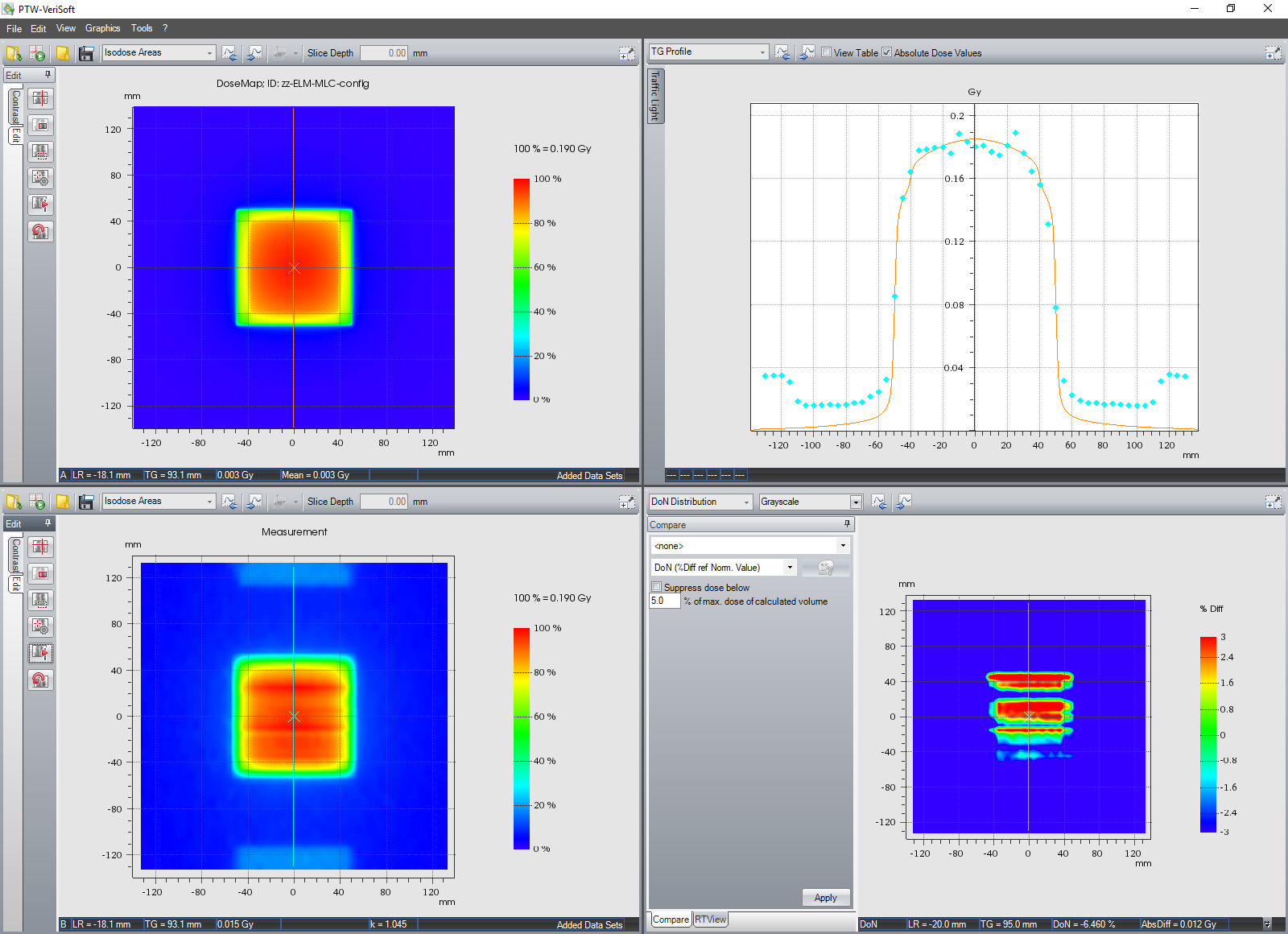
The transmission fields TrA and TrB have the lowest doses of all calibration fields. Due to strong local variation of interleaf leakage, fluctuations are high. Gamma tests are rather meaningless. However, the inplane profile is informative. "Smoothing by eye" is the recommended method to assess agreement.
The energy with the lowest transmission values of all is 6FFF. We first look at TrA, TrB, BLAU and GRÜN separately.
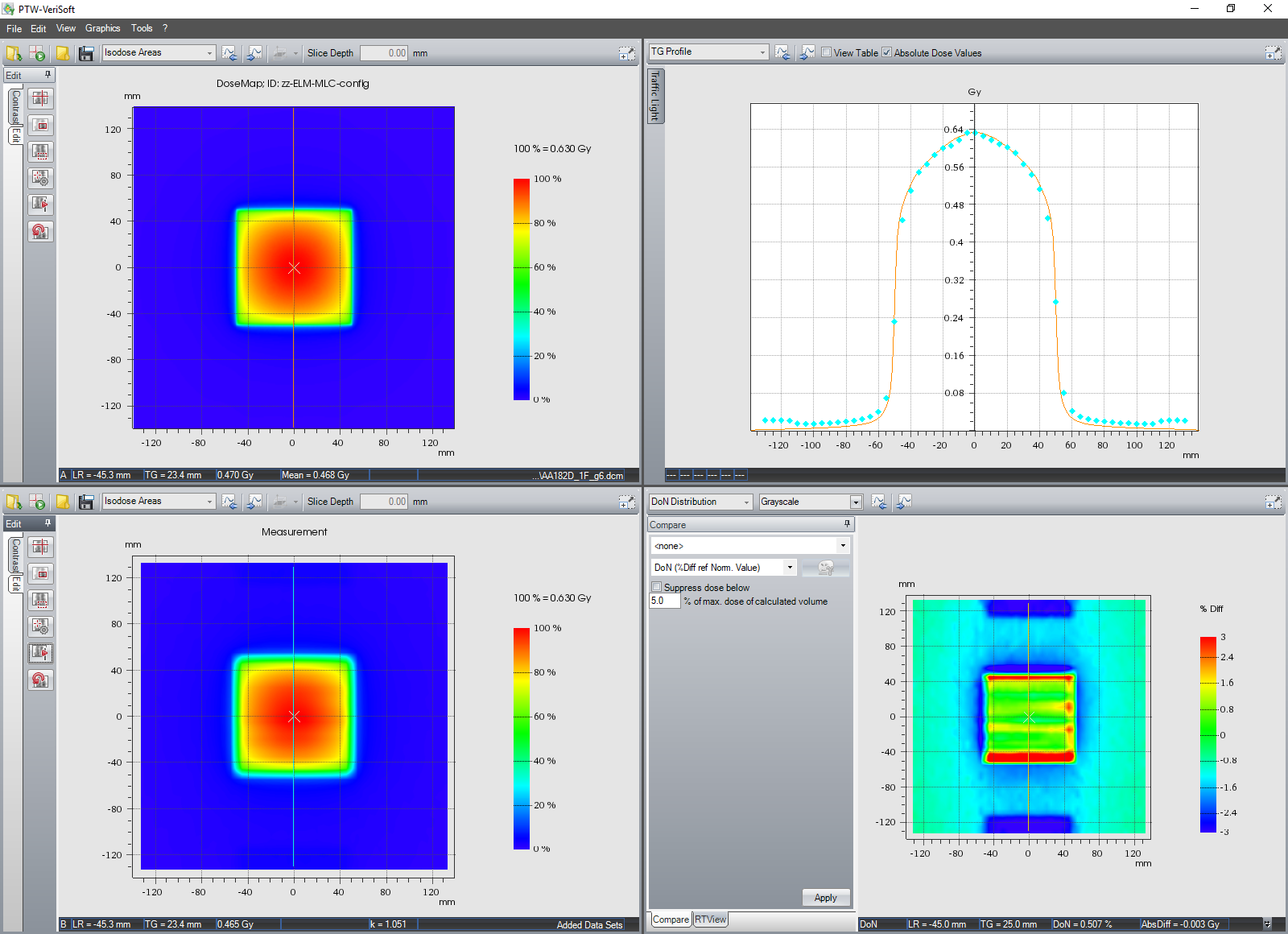
On the average, measured 2D doses (lower left) are reproduced nicely by the 2D-calibrated ELM (upper left)1:
(TrueBeam BLAU, TrA)
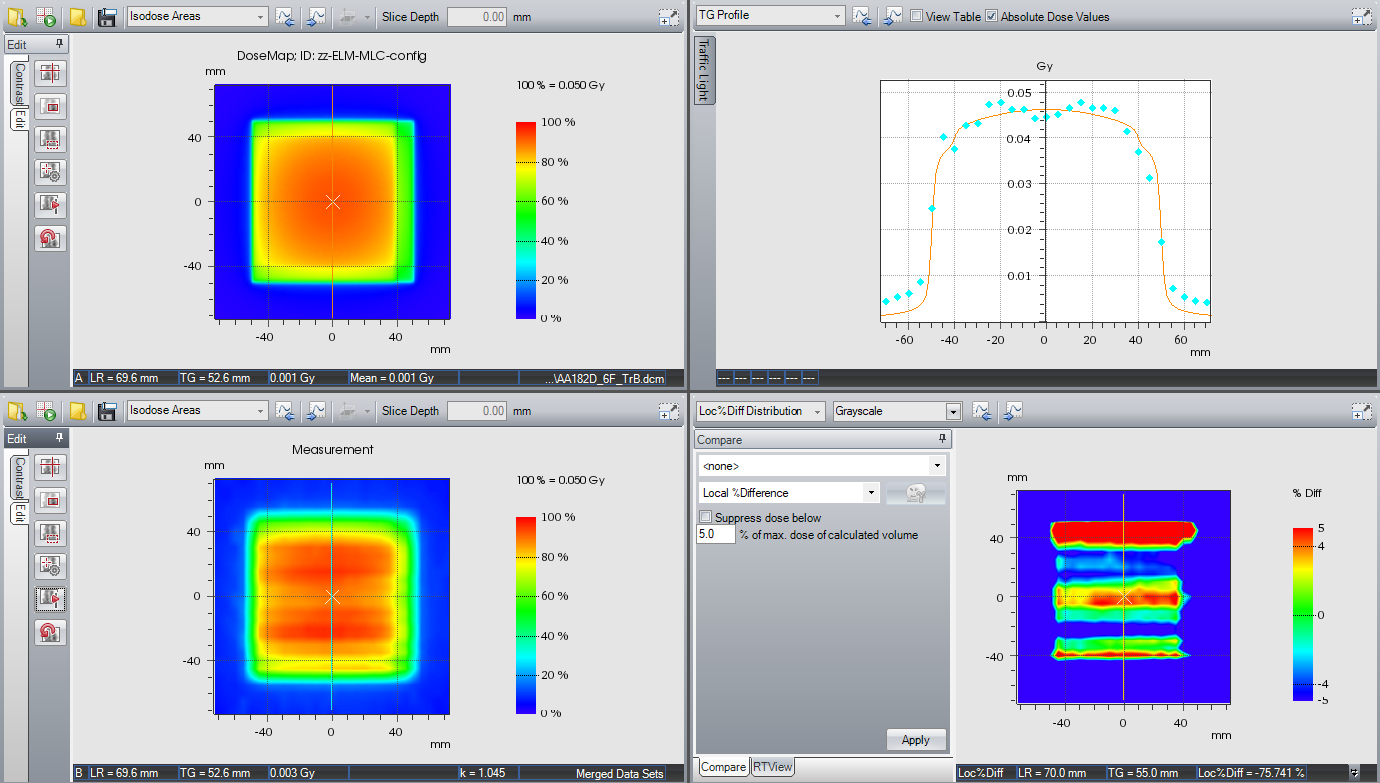
(TrueBeam BLAU, TrB)
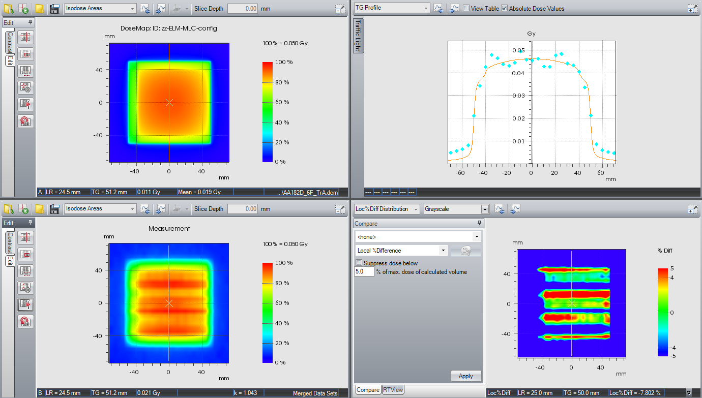
(TrueBeam GRÜN, TrA)
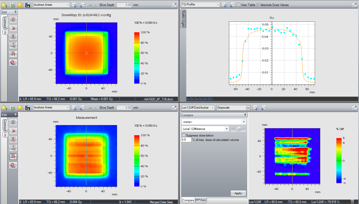
(TrueBeam GRÜN, TrB)
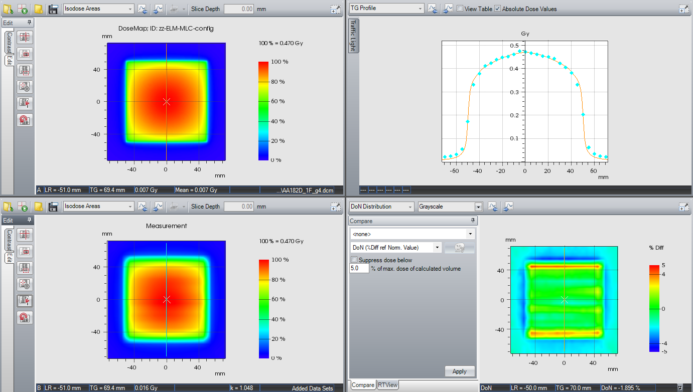
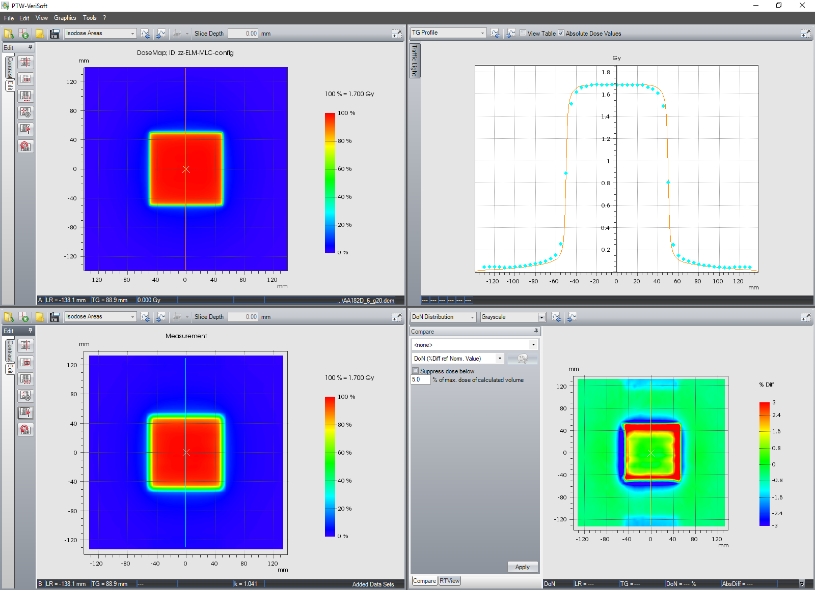
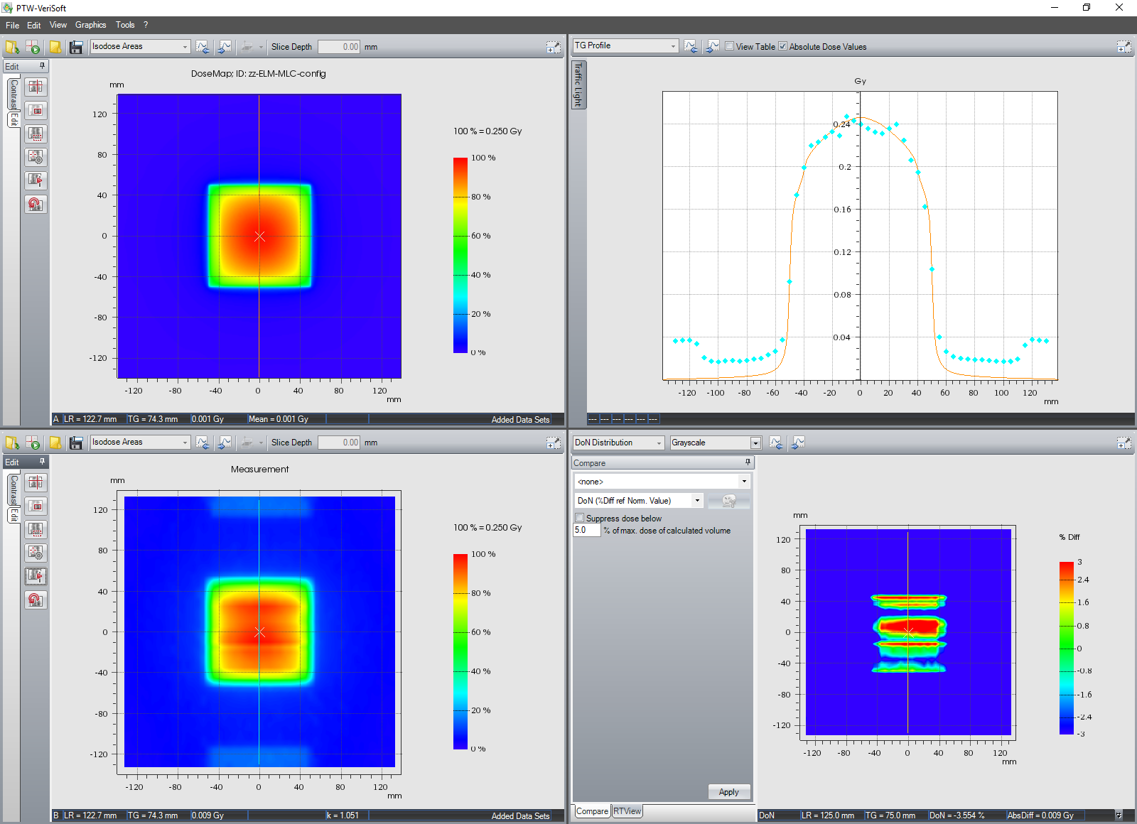
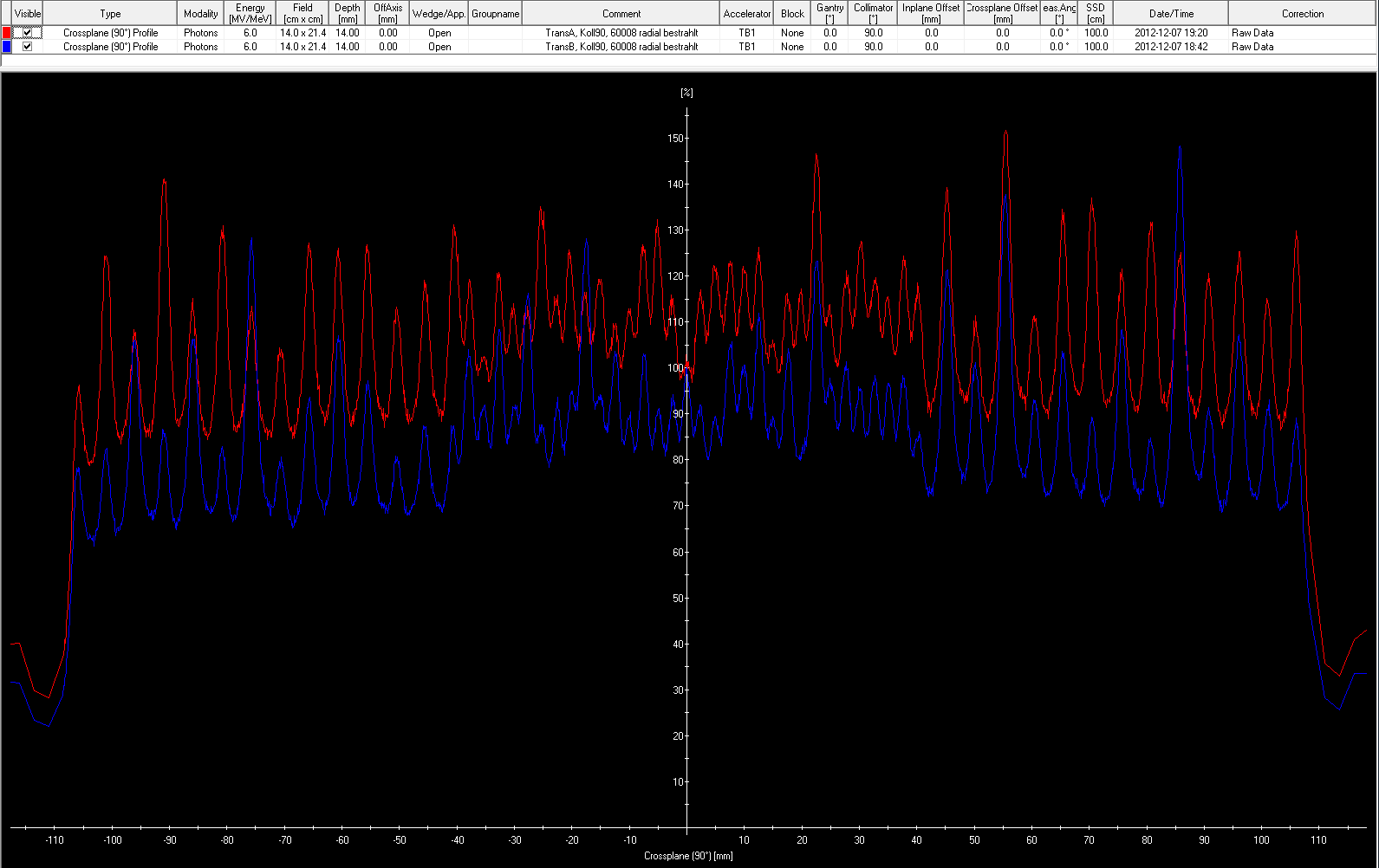
In VeriSoft, it is easy to sum up matrices simply by loading them simultaneously. Then they get added. This way, we can make all kinds of comparisons. We can, for instance, load on A (upper left) the calculated sum TrA + TrB, and on B (lower left) the sum of four matrices: TrA (BLAU) + TrB (BLAU) + TrA (GRÜN) + TrB (GRÜN). We still have to multiply matrix A by 2, but then we have the comparison, for the energy chosen, of calculated and average measured transmission, e.g., for 6X:
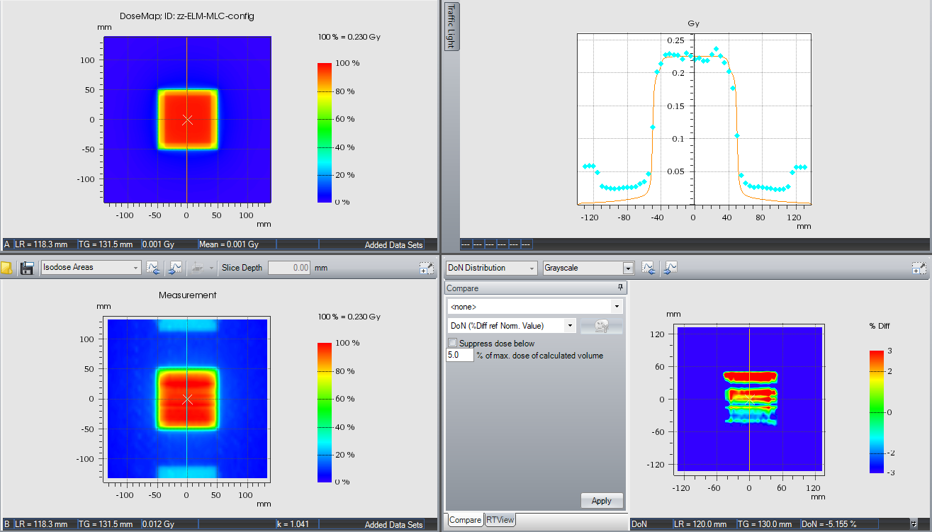
Matrix B and the disagreement outside the field in the inplane profile shown are clear indicators that there are some minor dosimetric effects that still need to be modelled in future releases of Eclipse.
Validation of Gap Fields
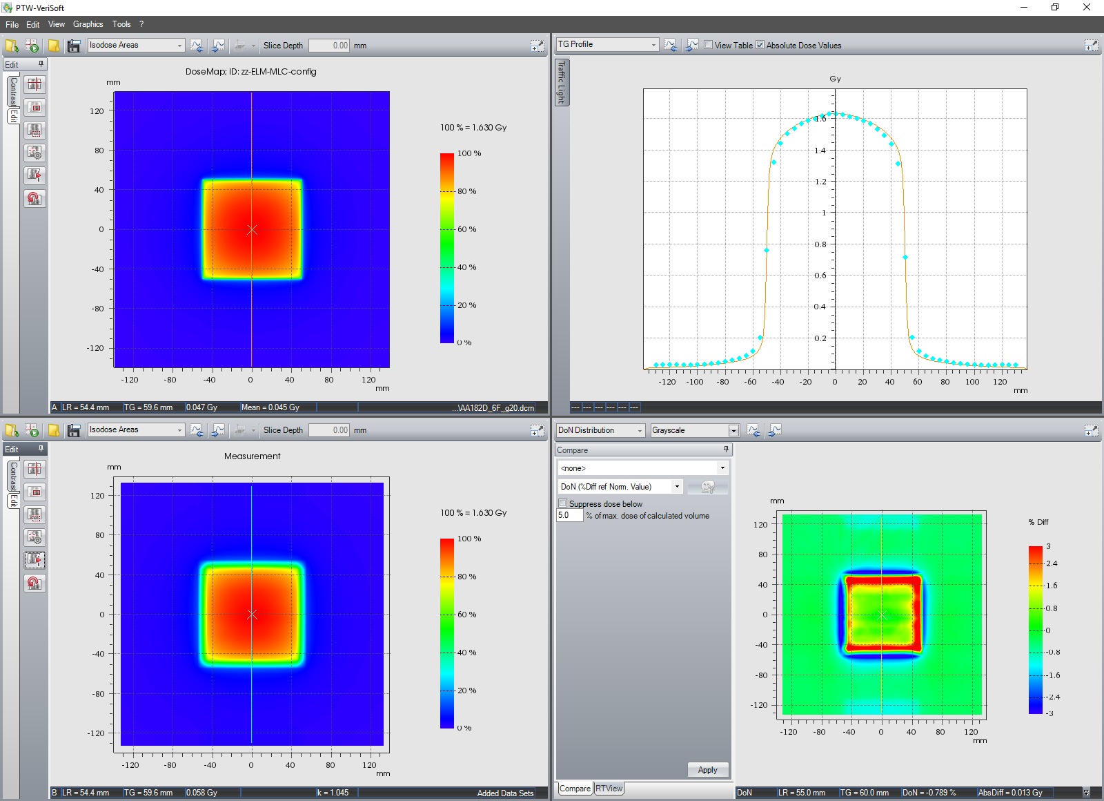
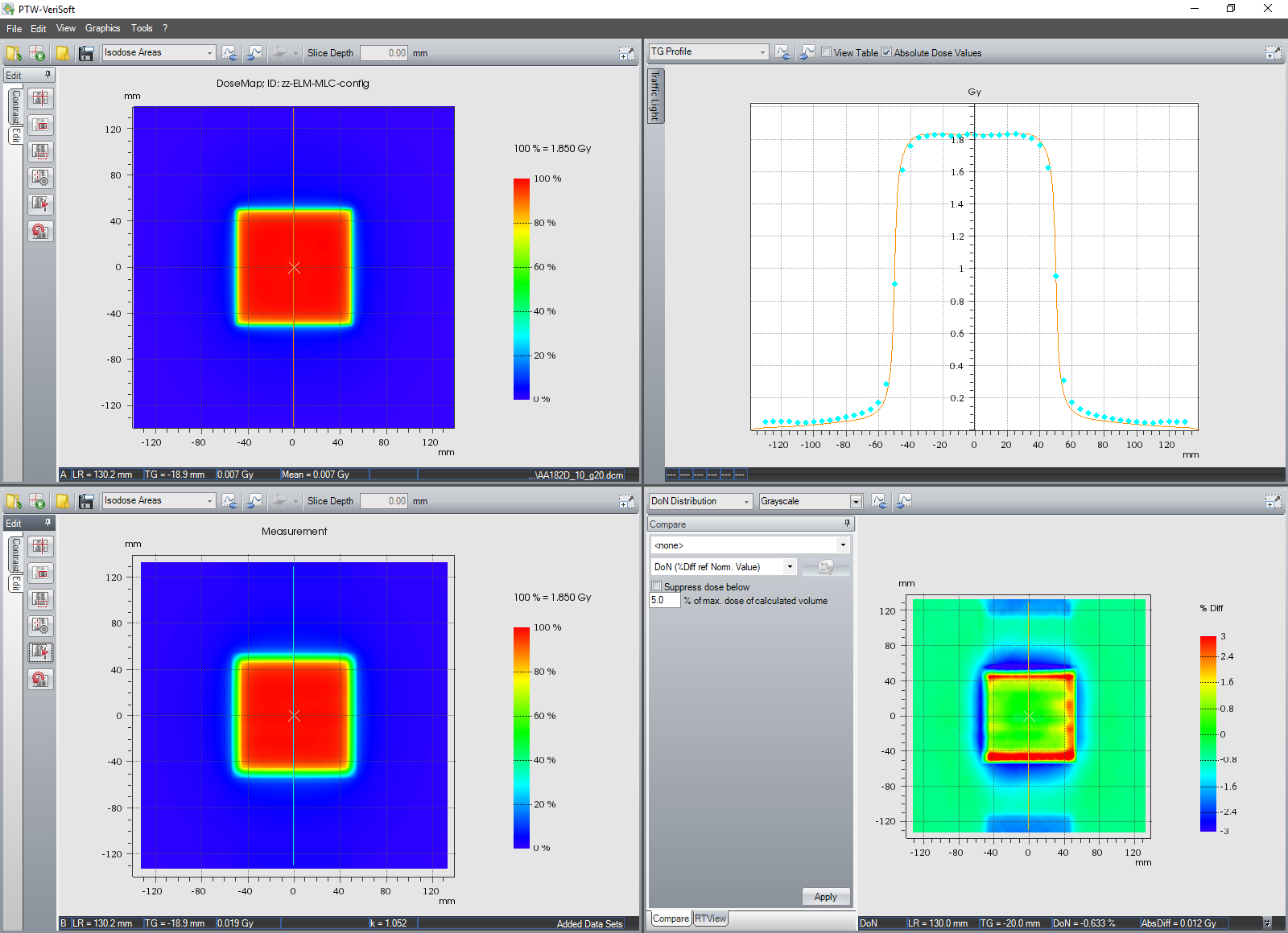
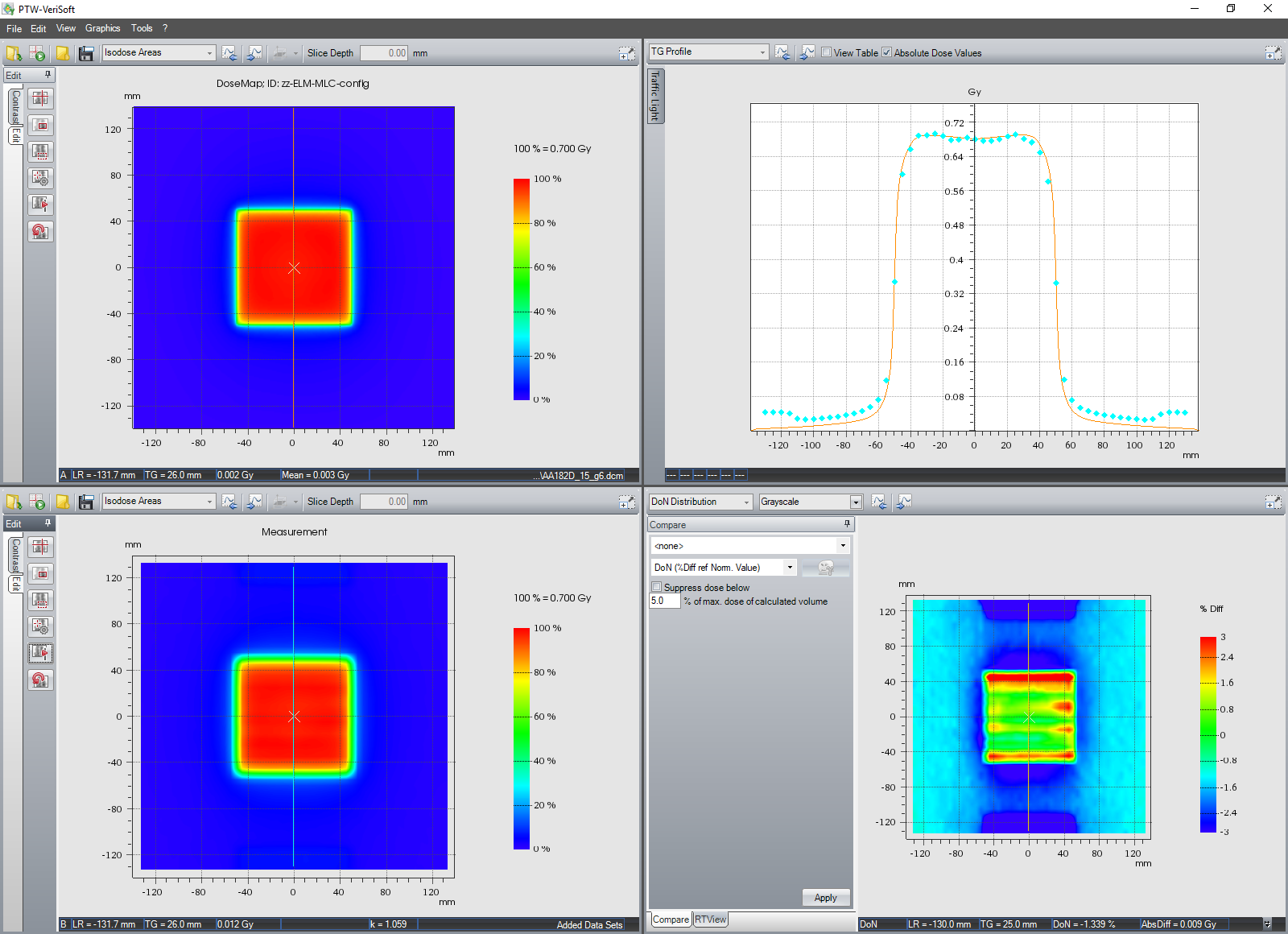
In the same way, we can validate the gap fields Gap4, Gap6 and Gap20. Here for instance the 20 mm wide Gap6 for 15X:

All validation comparisons (averaged machines, averaged Tr):
- 6X: Tr, Gap4, Gap6, Gap20
- 6FFF: Tr, Gap4, Gap6, Gap20
- 10X: Tr, Gap4, Gap6, Gap20
- 10FFF: Tr, Gap4, Gap6, Gap20
- 15X: Tr, Gap4, Gap6, Gap20
Some Final Thoughts
For the 50 comparisons, we found a very good agreement between ELM calculations and measurements. The check for "self-consistency" is also a good test whether something went wrong during ELM dosimetry configuration (typos, swapped digits, etc.). It is the same procedure as the verification of the Portal Dose Image Prediction algorithm (PDIP), where the treatment fields with the dynamic AIDA-pattern are delivered on the machine with imaging, the images are then used to configure the PDIP, and the PDIP is finally used to predict the images which already have been acquired:
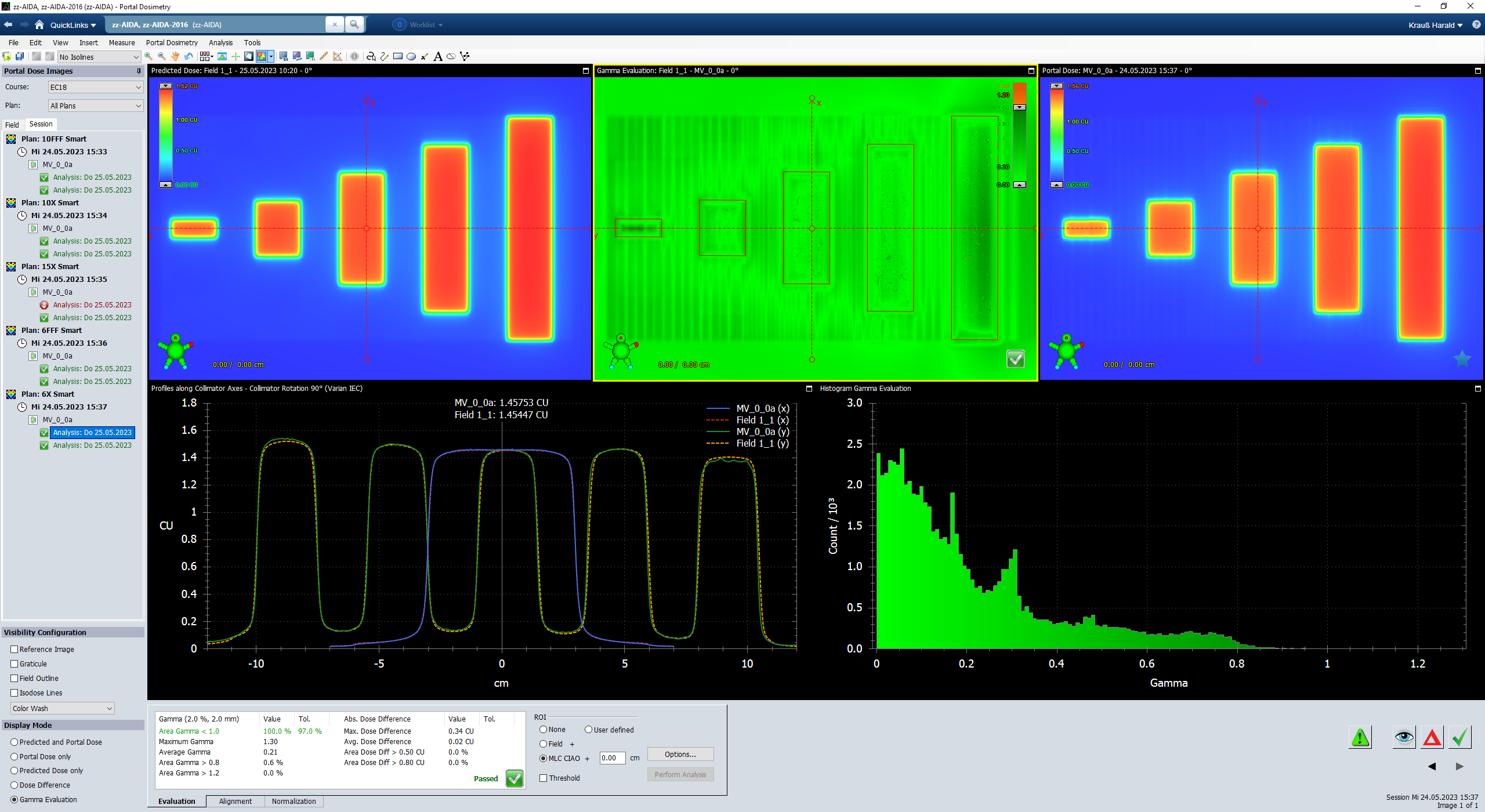
If the (earlier) acquired image more or less matches the (later) generated prediction, everything is fine.
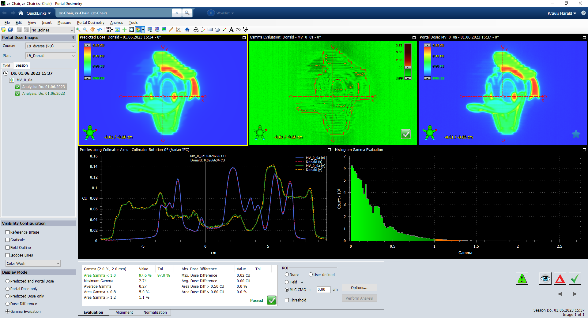
Once the validation for the calibration fields is done, one can try to verify more complex IMRT test fields, like this well known pattern. Due to the improvements of ELM, Donald easily passed the 2%/2mm Gamma test with a passing rate of 97.6%:
The 2D calibration method of the ELM is an interesting alternative to "Farmer" derived data. Besides the hopefully better quality due to the larger sampling area which should give more "representative" dosimetry values, there is also an educational aspect: Physical differences between leaf banks and between machines can be "visualized" as 2D patterns (dose distributions). By looking at these patterns (the horizontal stripes as shown in the screenshots), it becomes immediately obvious that, say, a certain leaf bank with a higher stripe density will also have a higher average transmission (compare TrB and TrA from above). This visualization is not possible when a single value is read from a dosemeter.
Small physical and dosimetric differences between leaf banks and between machines are a reality which has to be accepted. By looking at the 2D transmission plots or high resolution profiles, it becomes clear that further refinement of the ELM would have to address the separate modelling of interleaf and intraleaf leakage to a certain degree.
At the same time, such a refinement would immediatly be limited by the necessary "averaging" approach. The observed real leakage irregularities can probably never be modelled.
Temporal Stability
It should be kept in mind that each measurement is a snapshot in time. If we think of the MLC calibration as potential influencer, there is no guarantee that MLC dosimetry will remain stable over longer periods.
To get a feeling for the magnitude of variation we can expect, we remeasured (6X only) the six calibration fields after a PMI two weeks after the first data acquisition. In the course of the PMI on TrueBeam BLAU (#1275), an MLC calibration had been performed.
As expected, the measured values are slightly different. The largest change (0.5%) was found for the dose of the Gap4 field:
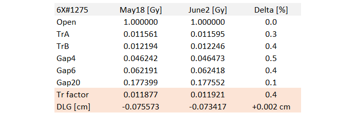
On the TBOX, separate AAA calculation models were created for the two data sets and the ELM dosimetry configured based on the measurements from May 18 and June 2. The results for Tr and DLG are highlighted in the table.
Visual differences in the transmission patterns can also be observed:
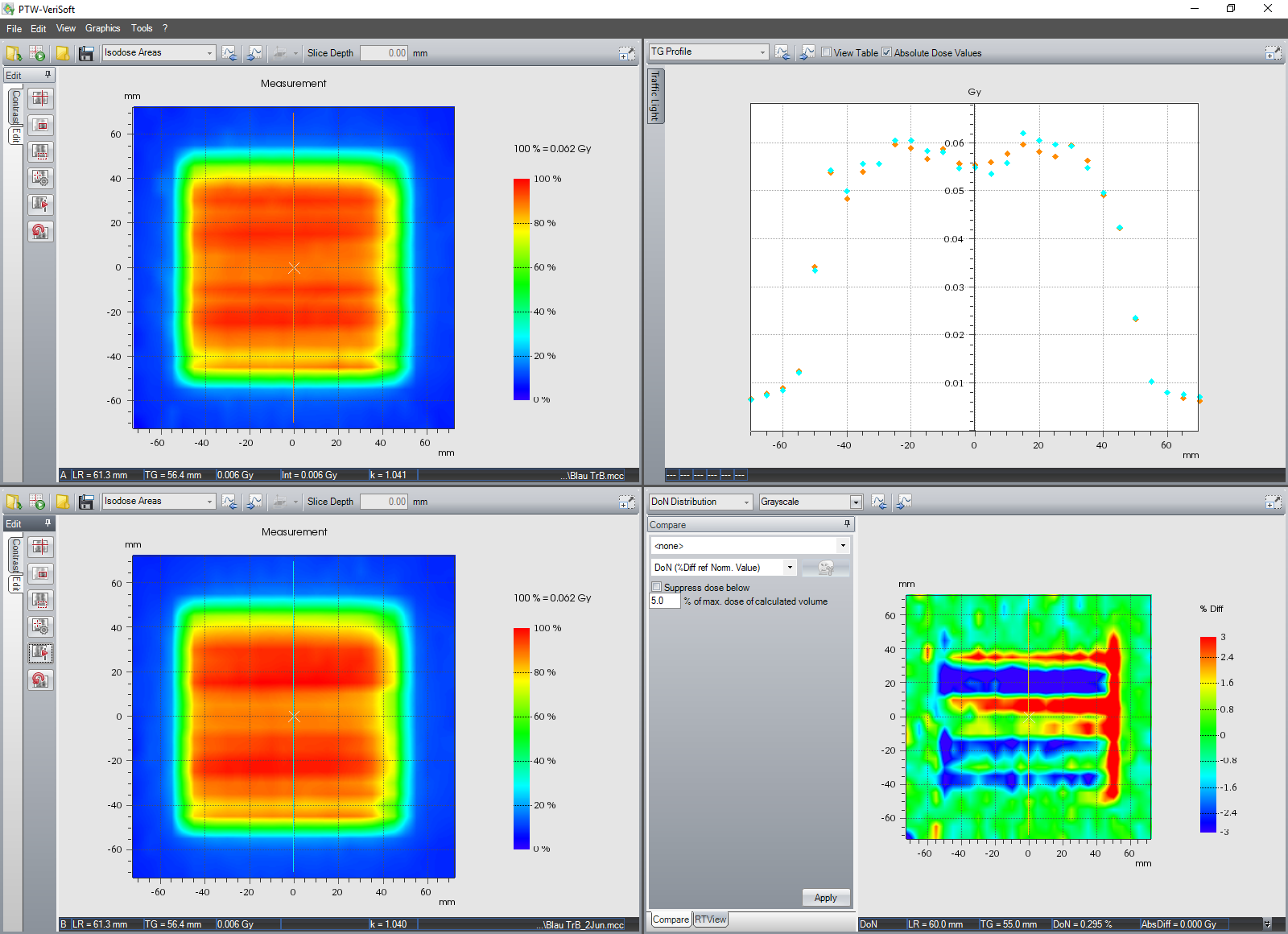
(TrA measurements from May 18 (upper left) and June 2 (lower left).)
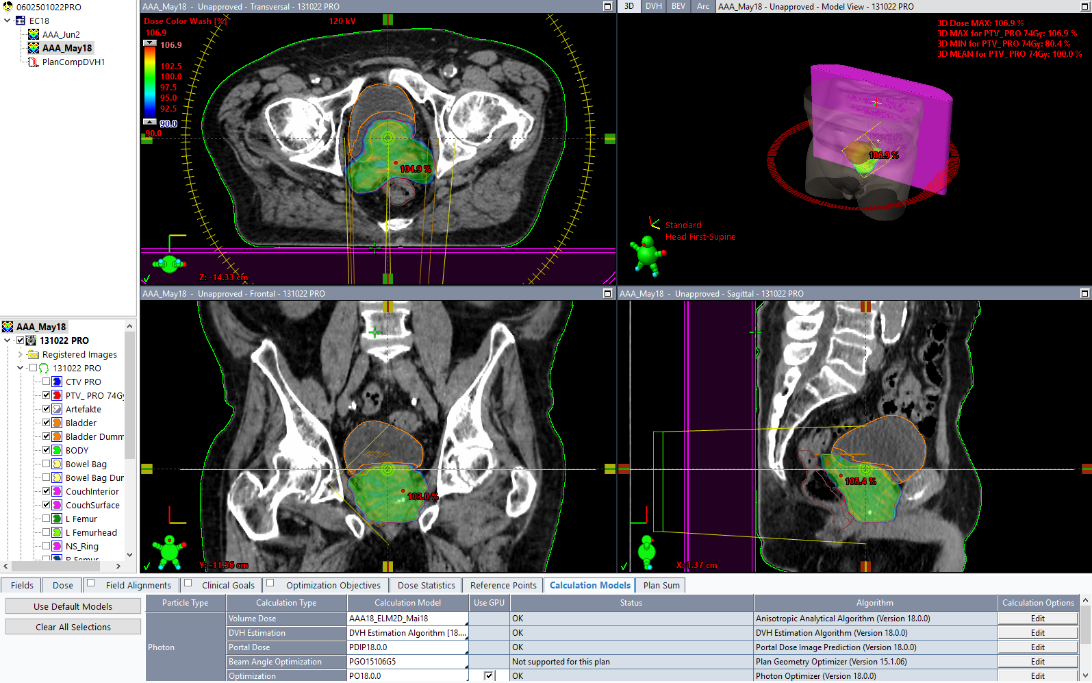
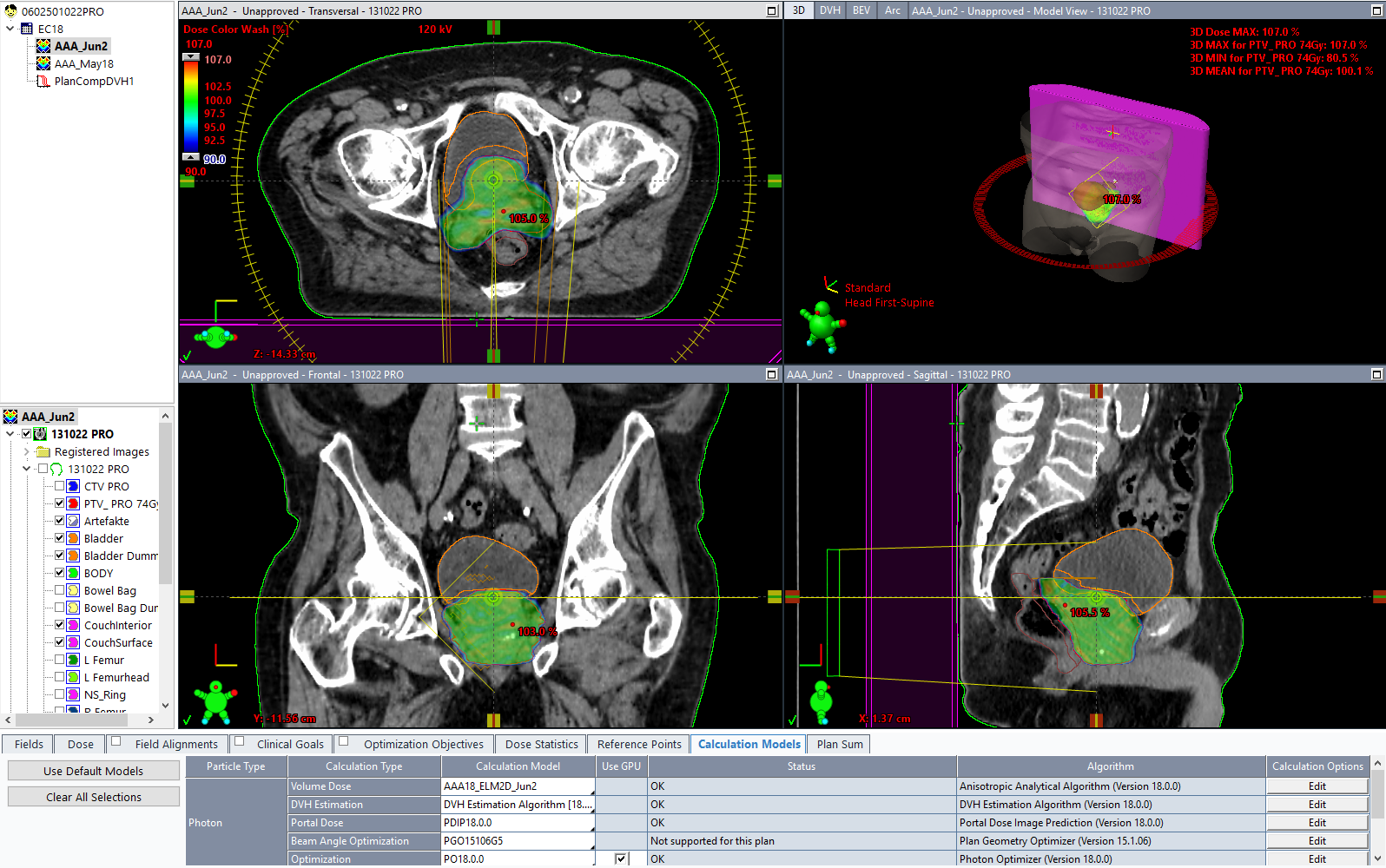
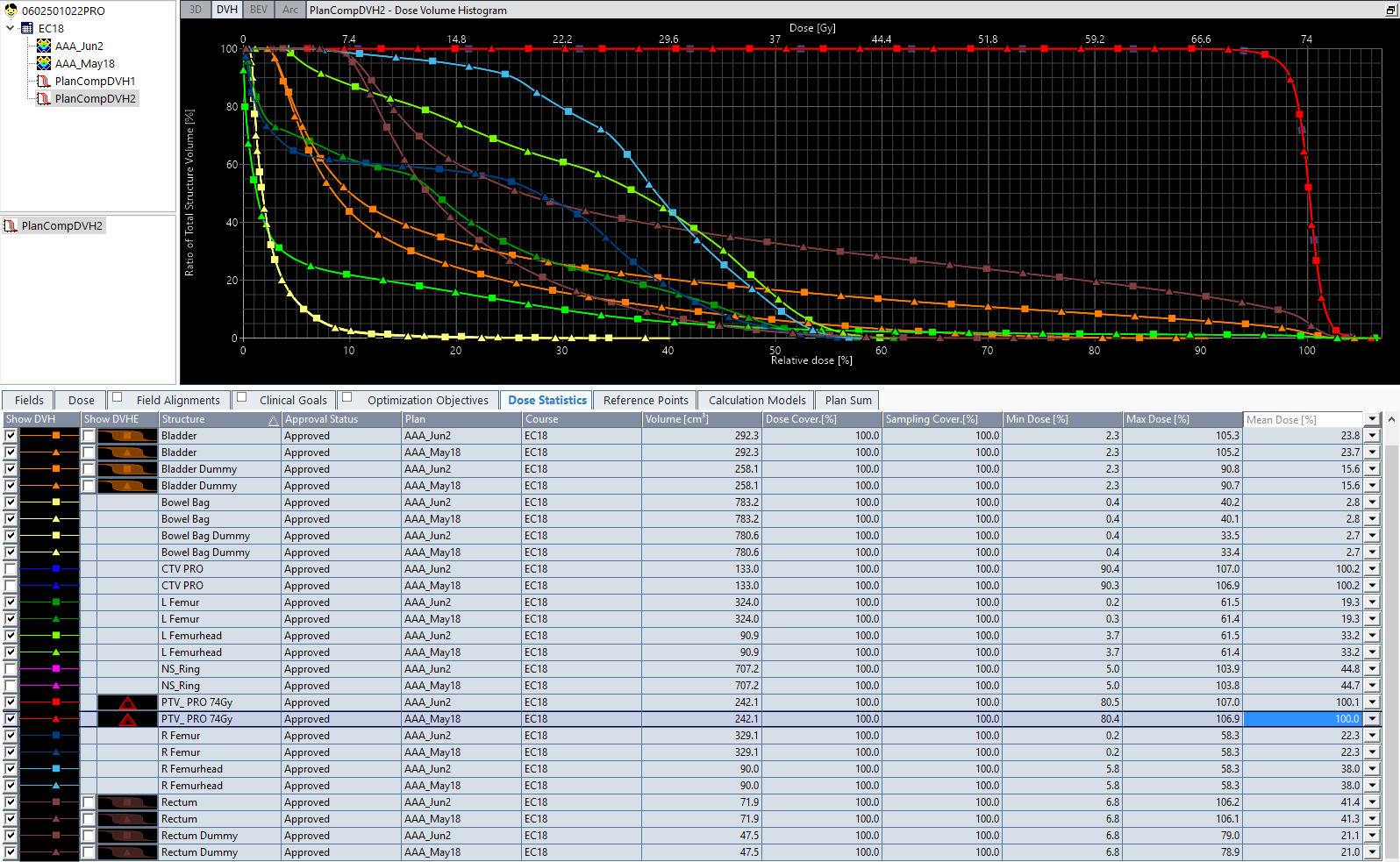
Would this change have an impact on patient plans? When the two calculation models AAA_May18 and AAA_Jun2 are applied on a typical prostate plan, the difference is negligible (target dose mean difference: 0.1%).
Nevertheless it is probably a good idea to establish a pattern of periodic constancy checks2 to make sure the ELM configuration is still valid.
Notes
1 Dose values in the VeriSoft profile plots, which are around 0.046 Gy at CAX, cannot be directly compared to the TrA and TrB values reported in Part I. Dose values for the Open 6FFF field are around 4.64 Gy at CAX.
2 One could, for instance, remeasure the Open + Gap4 field quarterly, and for a single energy only. This should give enough indication if the MLC calibration has changed.