
The latest version of Varian's treatment planning system offers several exciting new features and enhancements. We took part in what Varian now calls LLP1, which means that we were among the first who were able to use this release clinically. Configuration and testing started March 13 on the testing system (TBOX). First patients were treated on April 17 on the live system (ARIA 17).
Original and Enhanced Leaf Modelling
For the physicist, the most exciting new Eclipse feature is Enhanced Leaf Modelling (ELM), because it touches the physics of the treatment machine.
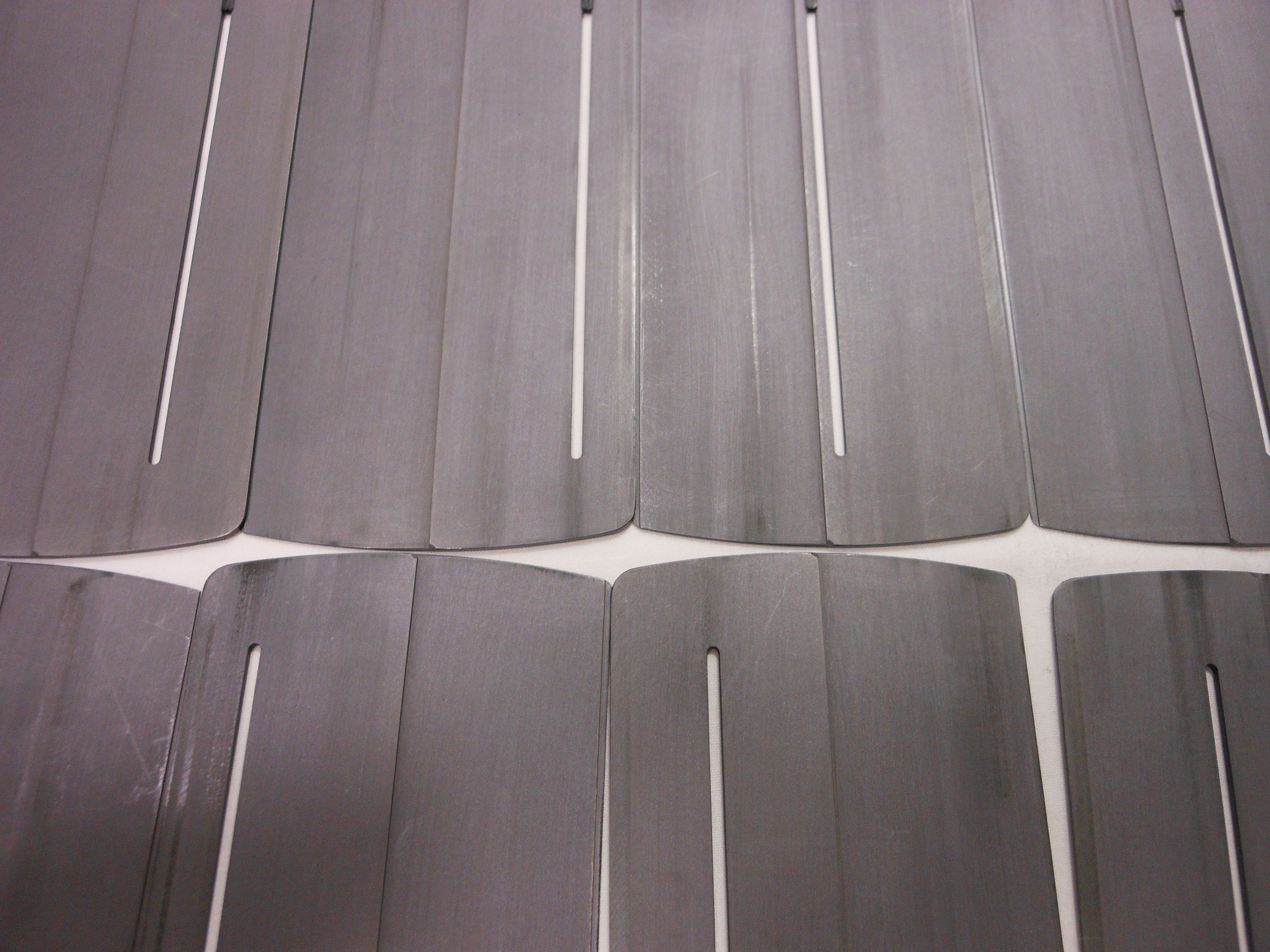
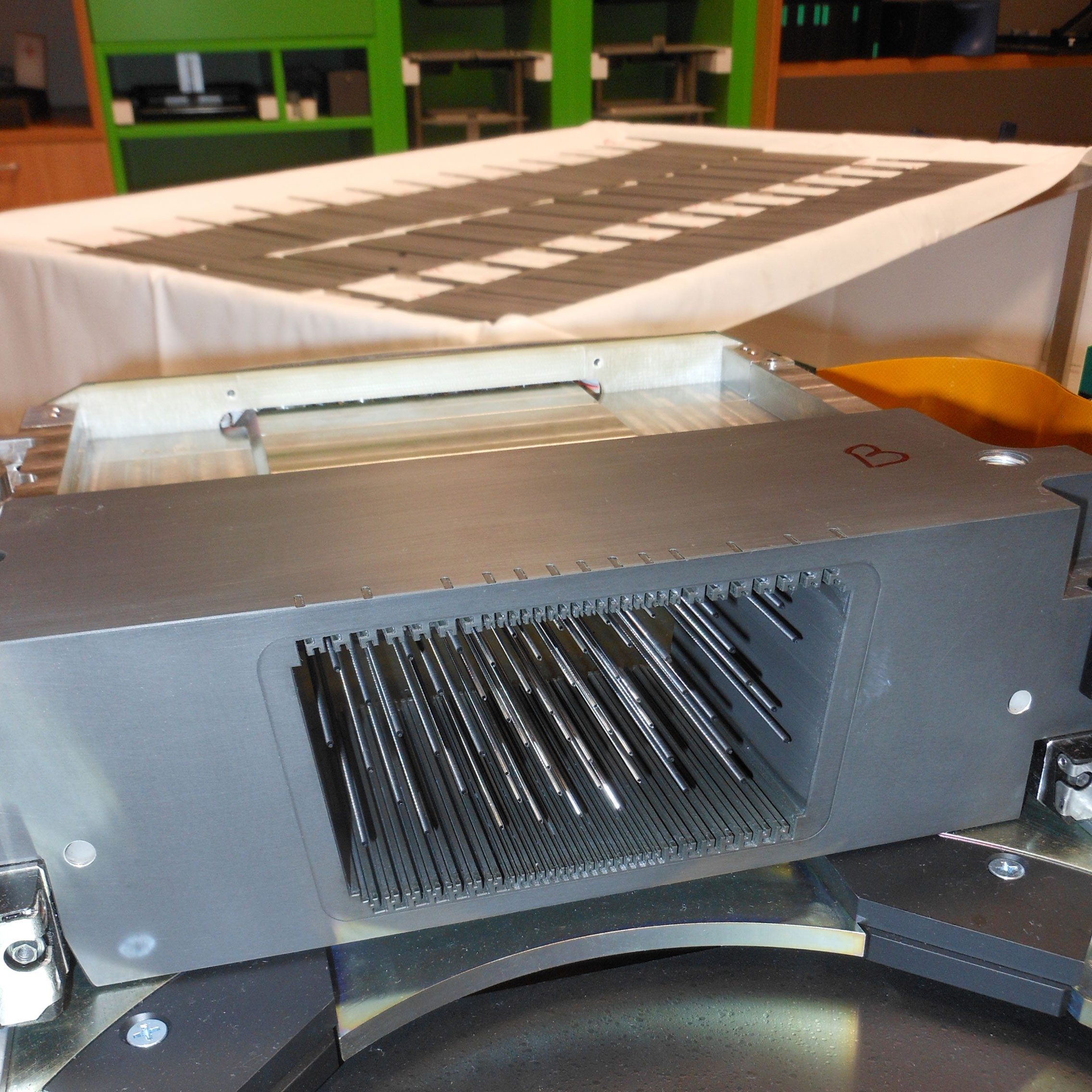
Up to and including Eclipse version 17, MLC leaves are modeled in a simplified way: The "original MLC model" (OMM) actually treats the rounded leaf tip (photo) as flat. This underestimates the fluence, if a certain leaf pair forming a (static or dynamic) gap is at an off-axis position. The fact that the leaf tip in reality is rounded is modeled in the OMM with the help of the Dosimetric Leaf Gap (DLG): for the fluence calculation, the distance DLG/2 is added to the leaf positions, which means that if a leaf gap is "closed mechanically" (leaf tips touch), it is "open dosimetrically" by DLG. Typical DLG values are around 0.4 mm for the HD120, depending on energy. See our article on the HD120 from 2013.
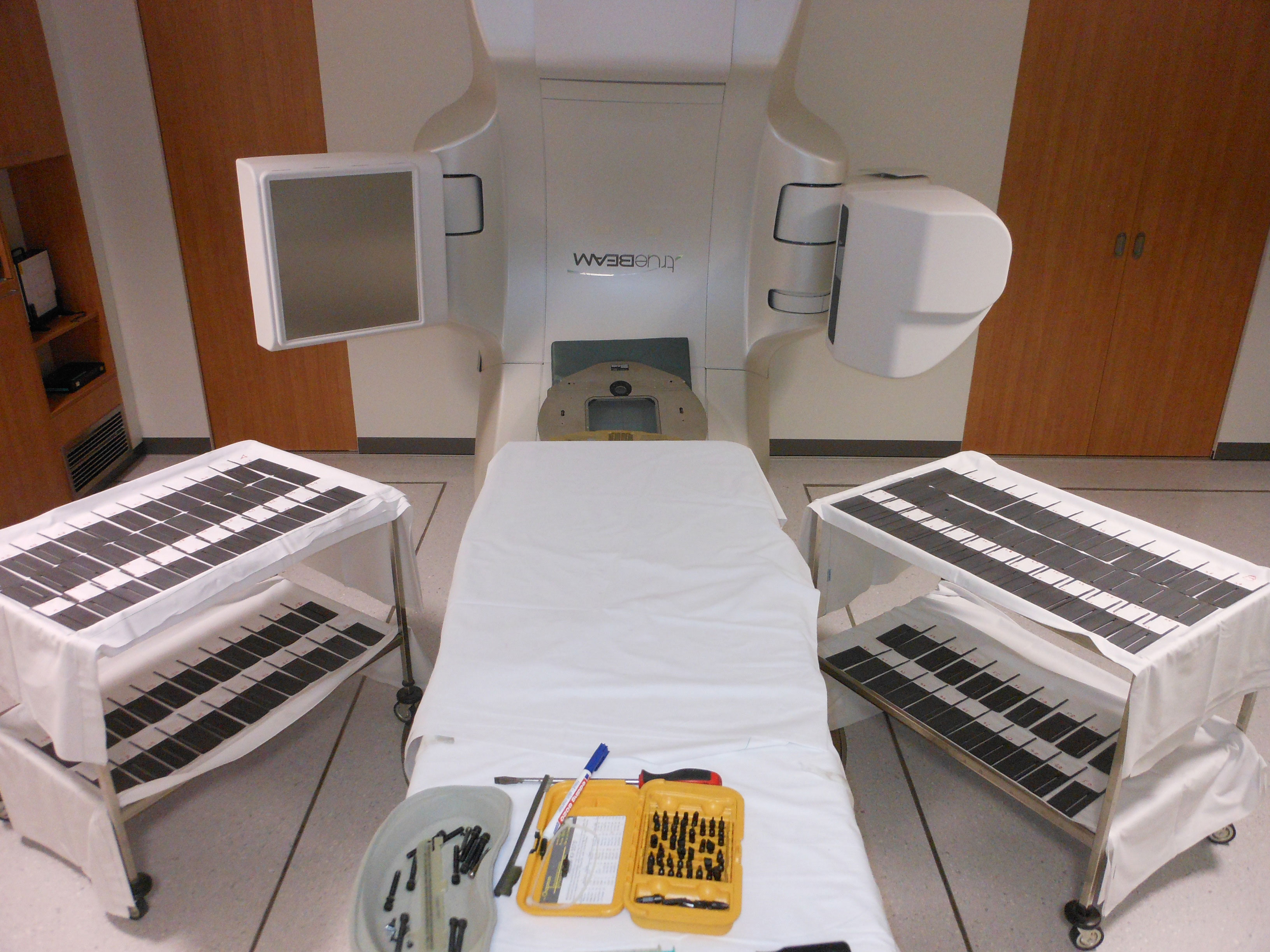
(For best modeling results, it is advised to clean all leaves before an upgrade to ELM ;-)
Another simplification of the OMM is to use a single transmission value for different leaf widths. Users of a HD120 will know that the quarter leaves (0.25 cm width), which cover an 8 cm long area in the field center, have a slightly higher average transmission2 than the off-axis leaves (0.5 cm width). When configuring the calculation models, one can only either focus on the central part of the field (by using the leaf transmission of the quarter leaves), or take an average of the transmission values of the two leaf types. A compromise in either case.
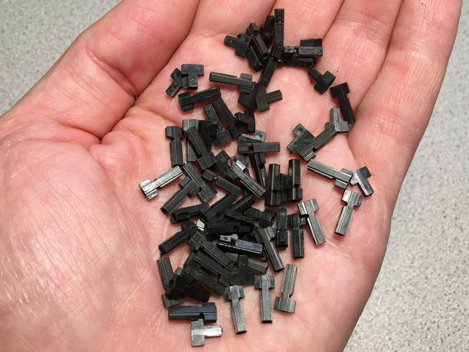
The third simplification is the assumption that the leaf is internally homogeneous, i.e., filled with material everywhere. In reality, each leaf has an cutout for the drive spindle (drive screw, see photo) which runs from the base to a point near the leaf tip: only the frontmost approx. 3 cm feature an uninterrupted cross section:
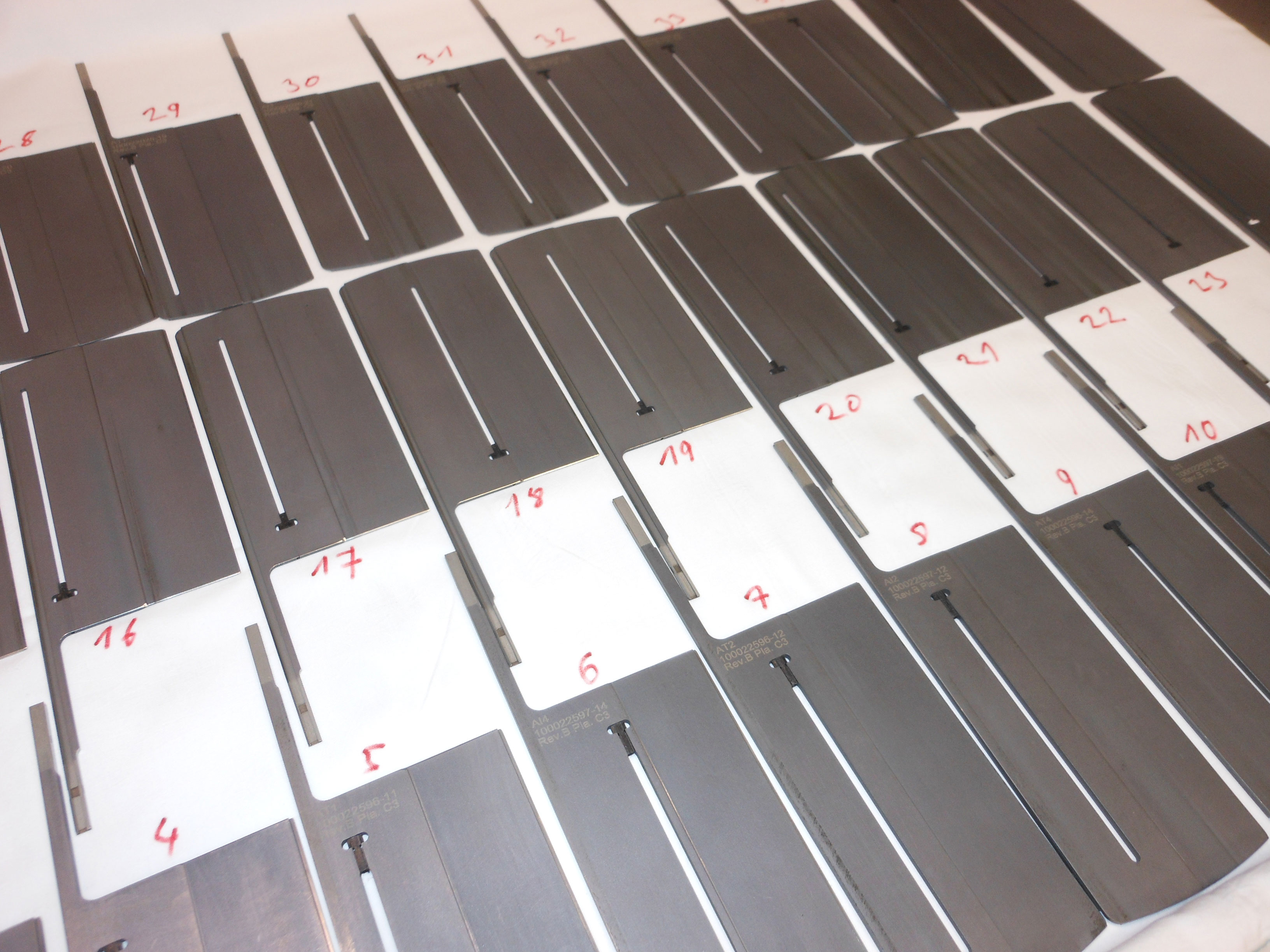
(Leaf features: curved front face, cutout for drive spindle, T-nuts)
The differences between OMM and ELM can be visualised by comparing AAA dose calculations of the two MLC models. Acuros XB (AXB) would give similar results, since both new algorithms take advantage of ELM.
Calculation Preview: Simple Static Test Field
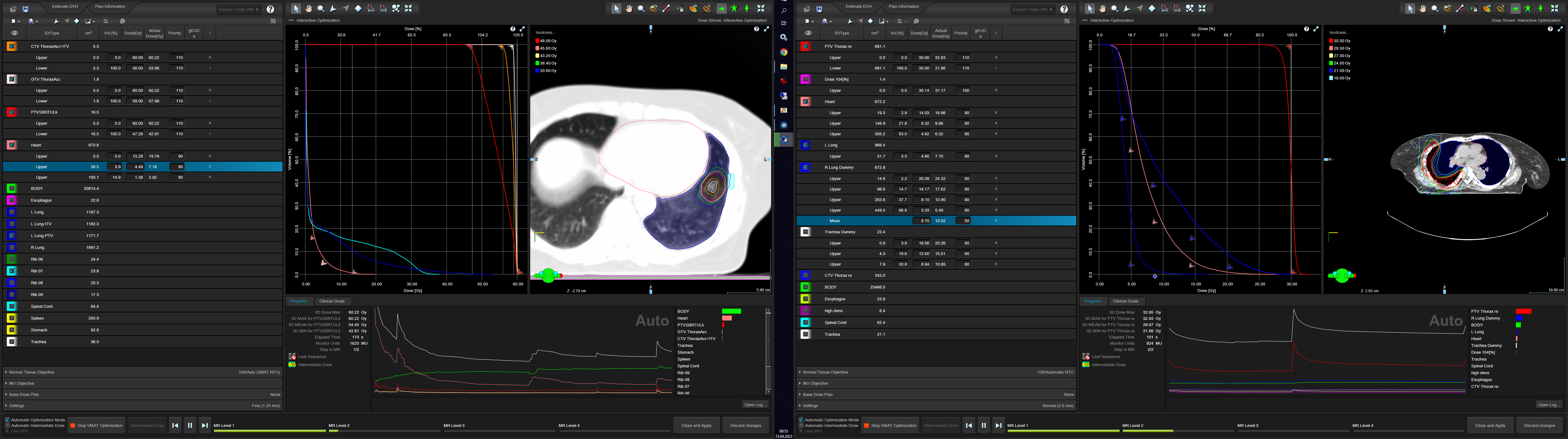
After ELM has been configured (see below), it can be used for dose calculations. A simple static 6 MV field has all leaves closed at centerline. The jaw setting (yellow frame) is 15 cm by 20 cm:
Dose calculation (grid: 1 mm) mainly reveals the transmitted dose through the centerline gap, but also the transmission elsewhere in the field.
SSD was set to 98.5 cm, so that the isocenter is approximately at dmax depth. Left is AAA16.1, right is AAA18:
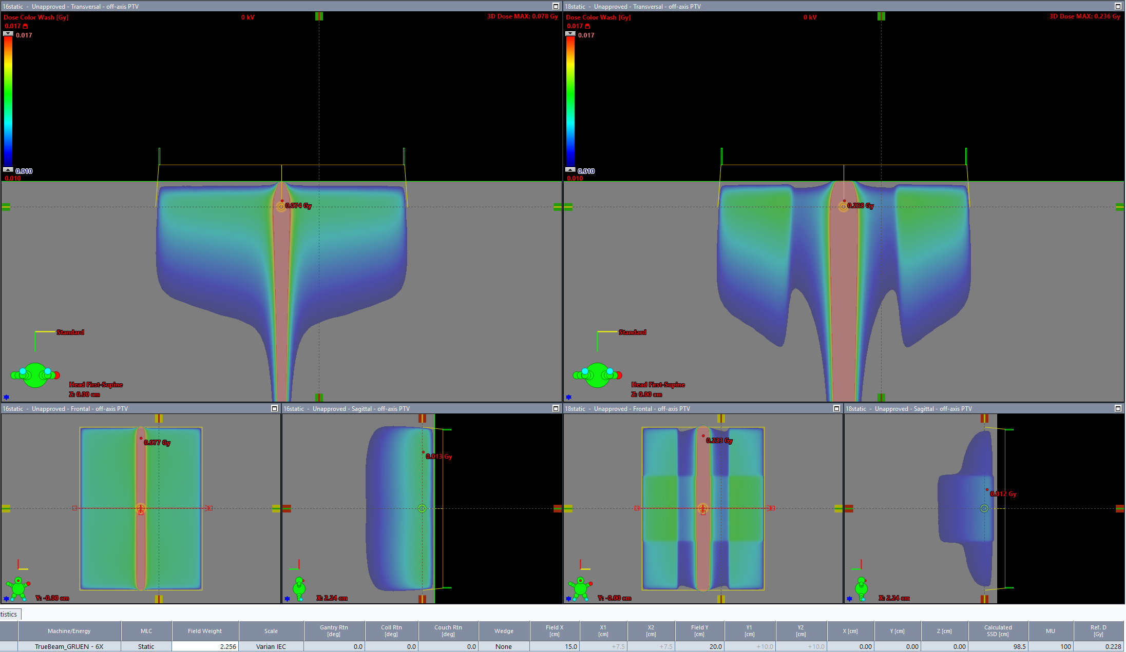
To amplify the differences in the low dose region, the colorwash scale was set to a low range (0.010 - 0.017 Gy). It is the same in both plans. However, the 3D dose max is different (upper right corners in red): for the OMM, max dose is 0.078 Gy. For the ELM it goes up to 0.236 Gy.
For the HD120 and ELM (right side, lower left view), the central 8 cm long region with the thinner leaves has higher calculated transmission than the thicker leaves, while for the simple OMM (left side, lower left view), all leaves are equal.
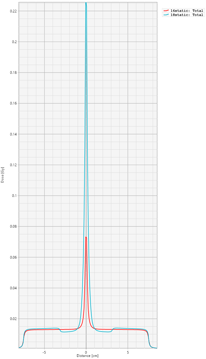
The next image shows the crossplane profiles through OMM (red) and ELM (blue) dose planes at isocenter. The profiles are quite different. ELM aims to model the true leaf shape. Due to the modelling of the rounded leaf tip, at centerline the transmitted ELM dose is much higher (click image to see full profile height), then drops to its lowest value (where the beam crosses full material), and finally rises again after about 3 cm from the leaf tip, because of the leaf screw cutout:
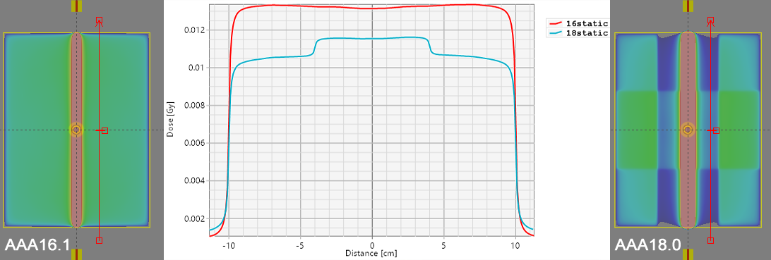
A longitudinal profile at about 2 cm off-axis reveals the difference between the different leaf widths once more. ELM models the thicker off-axis leaves with a lower average transmission. In the OMM (left), all leaves have equal transmission:
More on Transmission and DLG
The test fields which are used to collect data for the ELM dosimetry configuration are actually the same3 as for the OMM, only the interpretation of the determined parameters Transmission (Tr) and Dosimetric Leaf Gap (DLG) is different.
In OMM, the DLG covers the mechanical leaf gap of the MLC ("MLC calibration") and also includes the contribution of the rounded leaf tip. This part of the field (the penumbra region) can also be influenced by tuning the effective target spot size of the calculation model. After performing the measurements of the sweeping gap fields, the DLG value in OMM is obtained through extrapolation to gap width zero (see our article on the HD120), which combines the mechanical calibration and the leaf tip transmission in a single DLG parameter.
With ELM, spot size tuning is no longer necessary, and the "true" spot sizes may be used4. The changed interpretation of DLG is now that it still represents the mechanical leaf gap or MLC calibration, but not the dosimetric impact of the rounded leaf gap. That's why one should rather speak of the LG parameter, and not DLG. However, we will continue to use DLG, but we are aware of the new interpretation (In Eclipse Beam Configuration, the parameter is still called DLG as well).
What else is accounted for by ELM? Due to an attenuation model which is based on true leaf design (shape of the tip, drive train cutout) and divergent raytracing, ELM also considers the increased off-axis path length through the leaf material perpendicular to the direction of leaf movement.
The transmission value Tr is explicitely declared as the average transmission (averaged over inter- and intraleaf leakage) in the area around CAX and under the drive screw cutout (not the full material cross section), and the model takes care of the lower transmission under the thicker off-axis leaves.
ELM Configuration
As a first step, in Eclipse Beam Configuration, an ELM Multileaf Collimator Add-On has to be added to the Open Field, just like other Add-Ons such as the Enhanced Dynamic Wedge.
Under MLC Measurements, the measured values are entered. It makes no difference whether electrical (nC) or radiological units (mGy) are used, as long as units are used consistently. All values will be related to the open field:
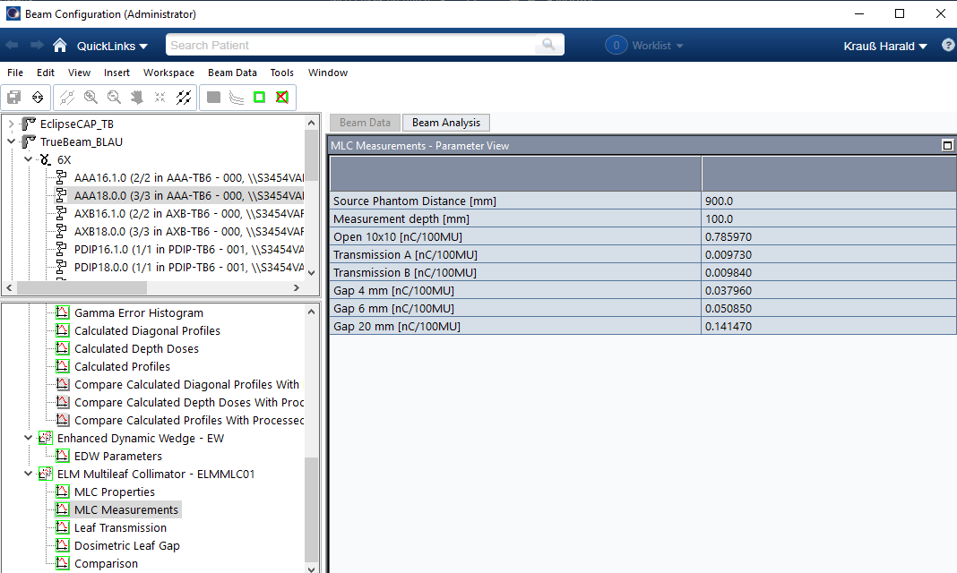
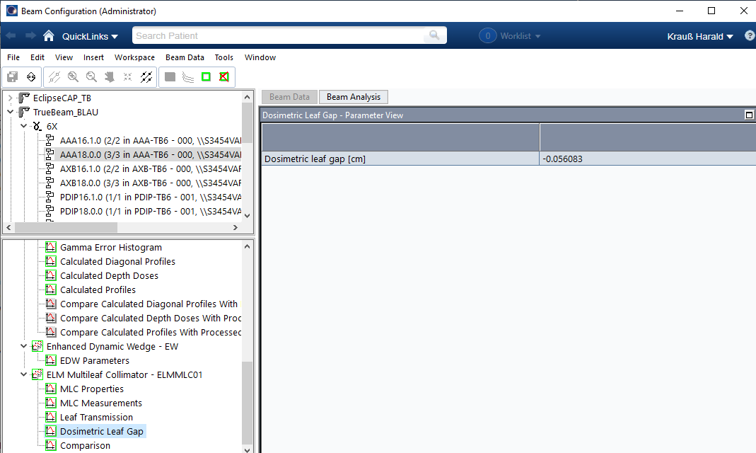
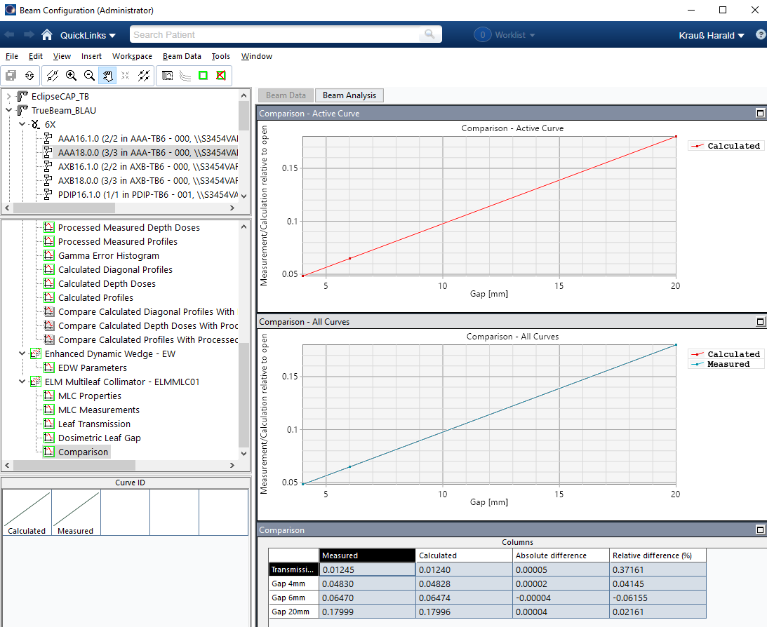
A configuration program then iteratively fits the data to provide optimal agreement between measured and calculated dose for the series of gap fields. Output are Leaf Transmission and Dosimetric Leaf Gap (the "new DLG" is now typically slightly negative), and a Comparison view:
Older MLC dosimetry values which are configured in RT Administration will be ignored by the ELM models, but should be left in place for older calculation models (up to version 17).
Comparison with Measurements
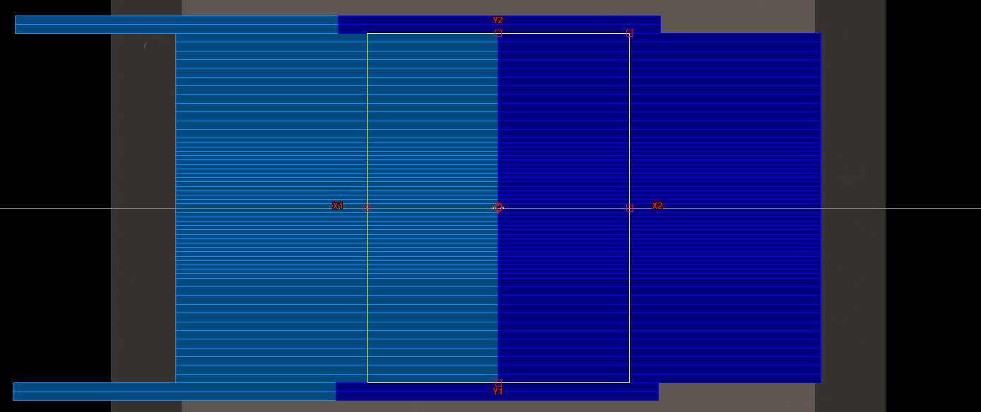
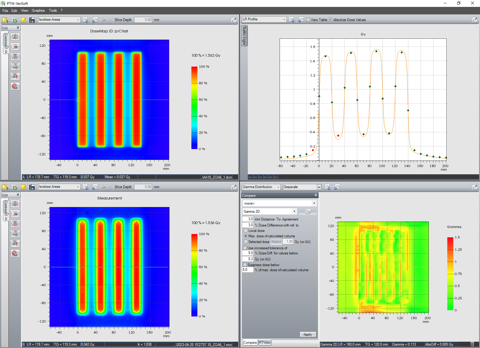
To give an overview which also shows the difficulties of the task at hand, we calculate, measure and evaluate a large off-axis 6 MV field which is fully blocked by the leaves of Carriage B. The field was calculated with AAA18, measured with the OCTAVIUS Detector 1500, and evaluated with VeriSoft 8.1:
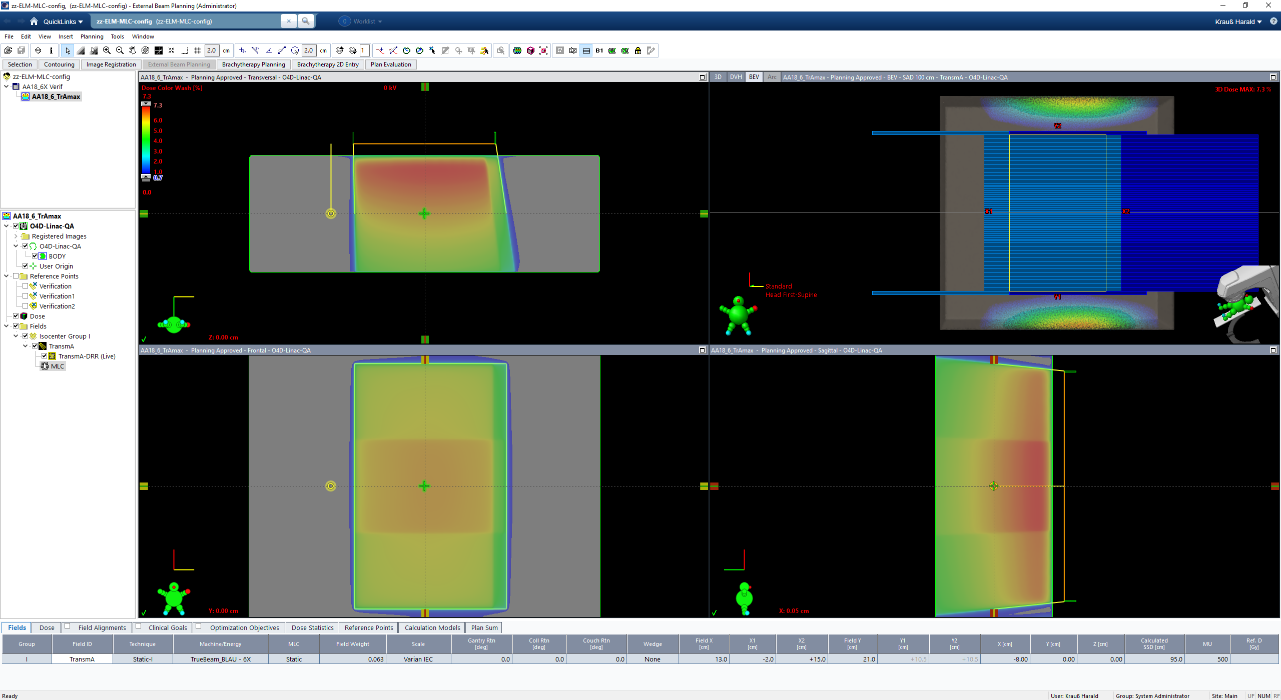
The X1-jaw is at -2 cm, X2 is 15 cm. Due to the low dose (about 0.07 Gy), the measurement is quite noisy (upper left is Eclipse dose, lower left is measured dose):
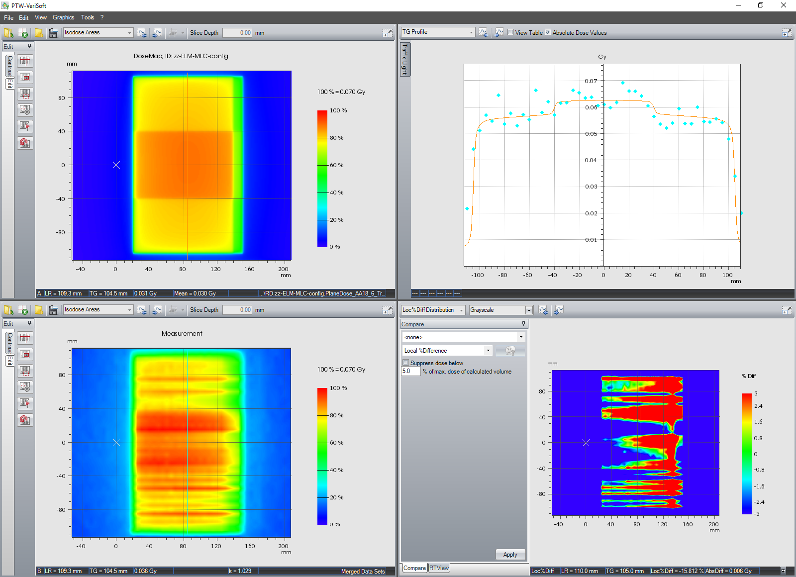
However, the longitudinal profile looks good, if averaging-by-eye is used.
Demanding off-axis fields with dynamically delivered zebra stripes can also be used to verify the ELM. Here, CAX is at the edge of the leftmost strip. The stripes are 2 cm wide. Between the stripes, leaves close dynamically because target fluence is zero. This field combines multiple aspects (Tr, DLC, off-axis agreement) of the ELM:
Test patterns are nice. However, the ultimate tests are patient plans.
Portal Dosimetry and ELM
We leave the world of phantoms and switch to Portal Dosimetry, which we use for 95% of all pretreatment verifications. We directly go to the other 5% - the most challenging plans: highly asymmetrical tangential IMRT breast fields reach from the central axis to nearly the edge of the 43 x 43 cm DMI detector. They are challenging partly because of OMM's simplifications.
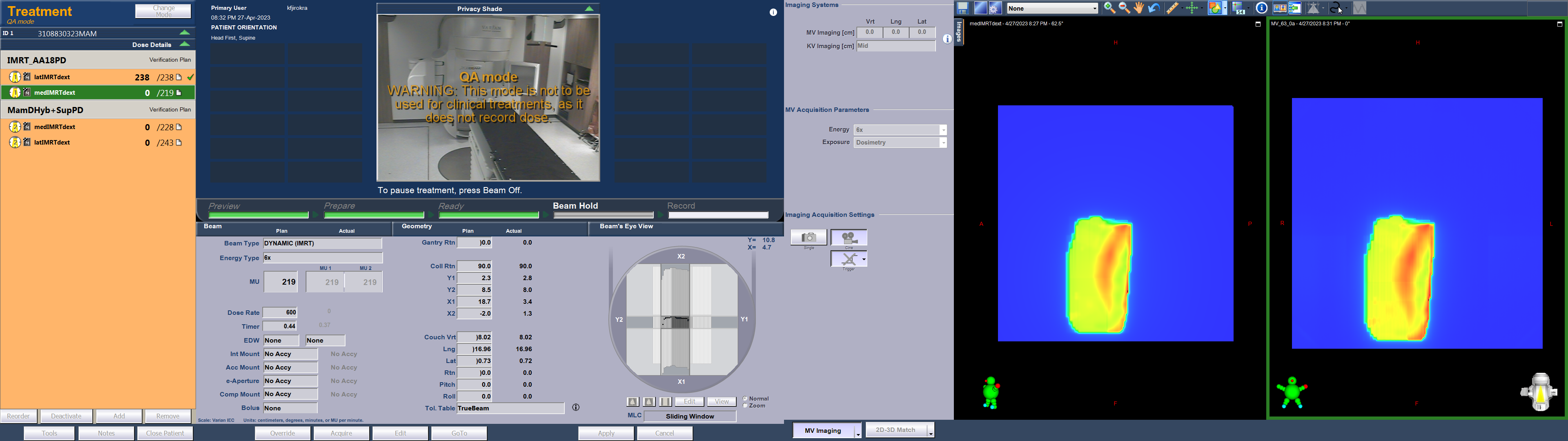
(This screenshot shows how close the field reaches to the detector edge.)
Since these fields usually don't pass our Portal Dosimetry Gamma tests (3%/3mm with a passing rate of at least 97%), we verify them by calculation, using Diamond software.
ELM interestingly has a positive impact on Portal Dosimetry as well, although PDIP is a simple 2D algorithm and neither AAA nor AXB are used. However, the PDIP algorithm takes the actual fluence as input, because by nature, it verifies fluence, not dose. And fluence, from Eclipse version 18 on, is ELM fluence.
The following patient fields, calculated with AAA16.1, had been mistakenly verified by Portal Dosimetry (PDIP16.1), with the expected poor result.
In the lower part of the inplane profile, one clearly sees the underestimation of the prediction (dotted red line), which mainly comes from the simplified leaf tip model in the OMM:
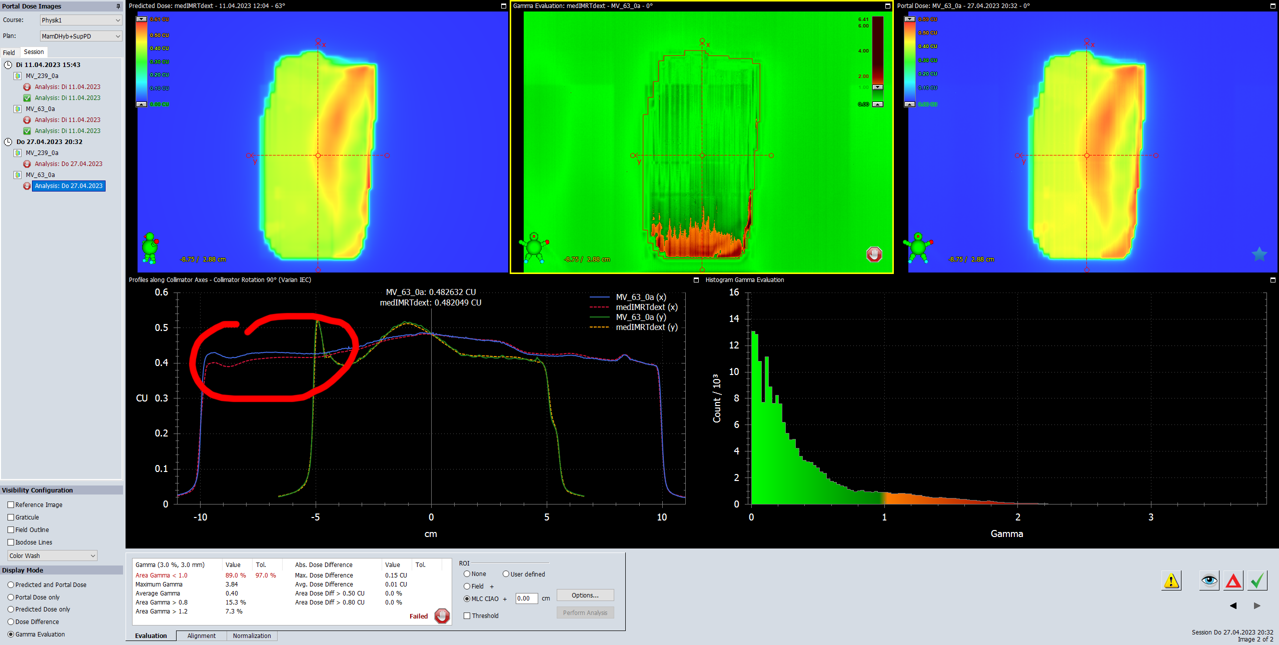
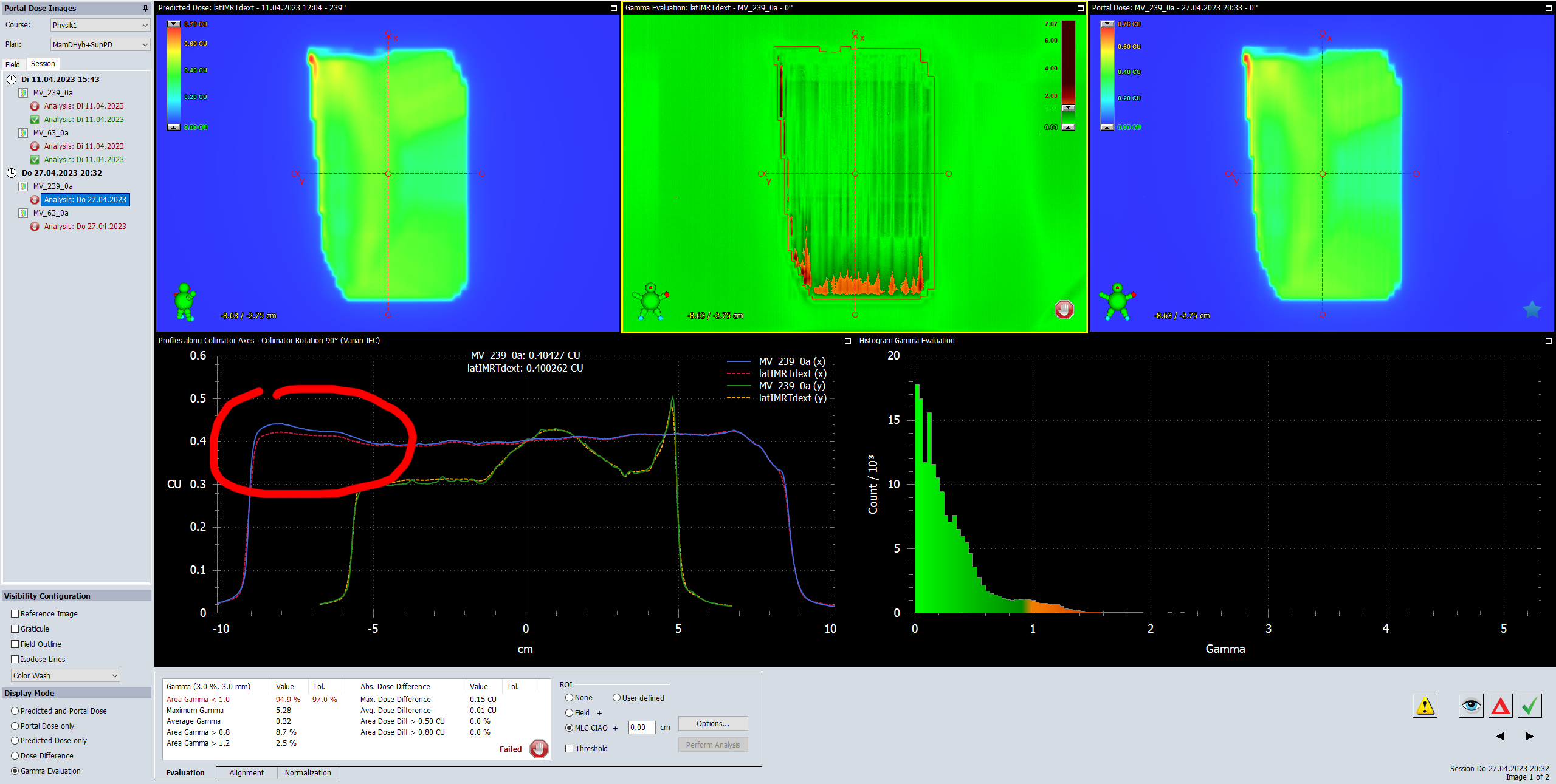
The passing rates for the medial and the lateral IMRT fields were 89.0% and 94.9% respectively, so the plan failed the test.
If one takes the same plan, switches to version 18 calculation models, re-runs the Leaf Motion Calculator (to take use of ELM) and repeat Portal Dosimetry, the results are much better:
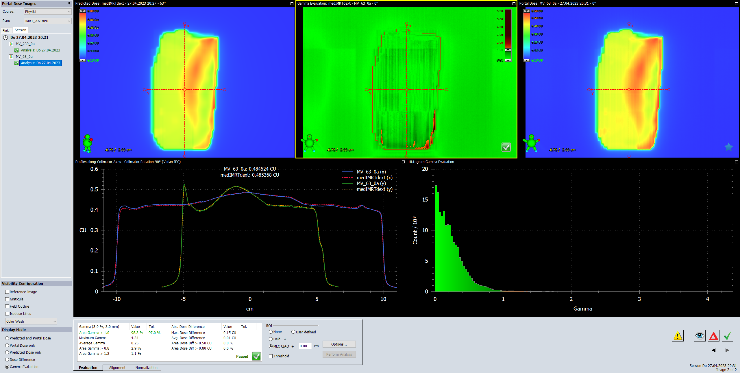
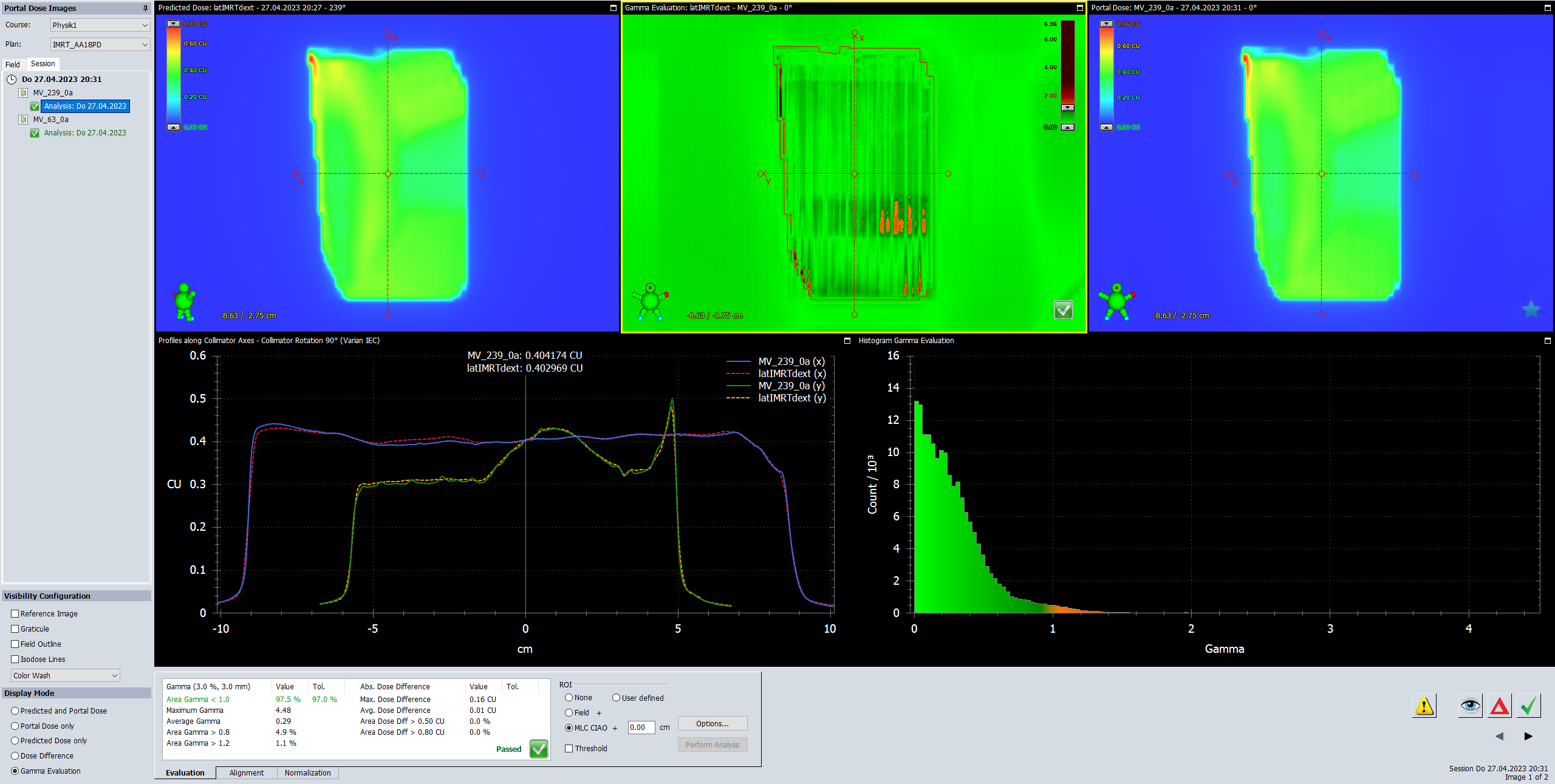
Passing rates are now 98.3% and 97.5%, and the plan passes the test.
We want to stress that ELM does not solve all Portal Dosimetry problems. The DMI is (still) no ideal 2D detector, and the half-beam intensity profile which is taken from a water phantom measurement at dmax depth and which is used to configure PDIP is another simplification. Nevertheless, ELM seems to have a very positive effect on the outcome of Varian Portal Dosimetry (VPD)5. Time will tell whether in the future, the challenging breast fields will as well be verified routinely with Portal Dosimetry.
Two weeks after upgrading to version 18, we can say that the improvements are really impressive!
Notes
1 The Limited Launch Plan (LLP) involves about five clinical centers. See also our testing of ARIA 15 in September 2016, when LLP was called CSCP.
2 Inter- and intraleaf lekage are not modeled separately. The input data for transmission (both OMM and ELM) is an average value. A larger volume ionization chamber, such as Farmer, is recommended for the measurement. The chamber does the intrinsic averaging.
3 They are static and dynamic 10x10 cm fields, centered around CAX. The only difference is that the number of dynamic (sweeping) gap fields has been reduced from seven to three (4, 6 and 20 mm gap width).
4 The recommended values for the HD120-MLC are SpotX=0.0 and SpotY=0.0 mm for AAA, and SpotX=0.5 and SpotY=0.7 mm for AXB, if ELM is used.
5 The other way to evaluate the DMI images, which uses EPIQA, benefits from ELM even more, because EPIQA takes the AAA calculated dose from Eclipse, 3D calculated in a slab of water.