Deconvolution qualitatively decreases the penumbras of a typical clinical measurement, increases the peaks and makes the valleys deeper. But can the measured deconvoluted profile be verified more quantitatively?
First we have to find a way how a David measurement can be predicted.
The idea is to find a suitable 2D-distribution and to calculate from this 2D-distribution how the 1D-measured David profile should look like. (It is not intended to predict the absolute signal, rather the relative distribution.) Ideally, finding a match between the calculated and the (deconvoluted) measured profile would be closing the gap between the TPS and David.
By calculating the line integral along each travelling leaf pair (with the summation of lateral pixels in order to reflect the MLC resolution), it should be possible to convert the "candidate" 2D-distributions to 1D-"David predictions".
What are the potential candidates?
Candidate 1: Optimal Fluence
The paper of Looe et al describes the radiation field hitting the David chamber in terms of fluence. Fluence is a quantity which is also present in the Eclipse TPS:
- Optimal fluence in Eclipse is the output of the inverse planning module. It is an "ideal" 2D-distribution which is not yet processed by the MLC sequencer module (in the case of Varian: the LMC - Leaf Motion Calculator). But optimal fluence is "aware" of leaf width (1 cm in our case).
- Actual fluence is the fluence which is actually leaving the MLC. It includes the physical limitations of the MLC, the most important being the static leaf transmission and the Dosimetric Leaf Separation (DLS). In actual fluence distributions, no pixel within the Complete Irradiation Area Outline (CIAO) can have zero value, because there is always some transmission present.
Optimal and Actual Fluence
For a sample 5-field anal cancer IMRT plan, the optimal fluence of the 320° field looks like this (click to see full screenshots):
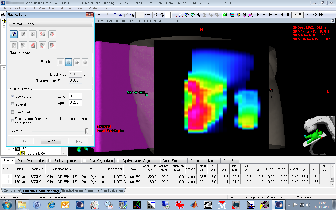
The optimal fluence matrix of each IMRT field can be exported from Eclipse as a text file with the extension "optimal_fluence". Its dimension and position can be found in the file header. The pixel size is 2.5 mm * 2.5 mm. Therefore, 4 neighboring pixels in each column can be combined when calculating the line integral per 1 cm wide channel in the David prediction.
The actual fluence is physically more realistic. As already mentioned, there are no zero pixel values within the CIAO region of the field, since there is always a certain amount of radiation transmission through the leaf body and the rounded leaf ends (which dominates the transmission through moving closed leaf pairs).
Other effects, like the splitting of large fields into "carriage groups" due to the mechanical travel limitations of the MLC are also reproduced by the actual fluence. There is no sharp border between the carriage groups, rather a broad overlap region, visible as horizontal strip in the middle of the field:

The 320° example field has two carriage groups. The actual fluence of such a field can be displayed for each carriage group separately, or as combined "total actual fluence" (as displayed in the screenshot).
Unfortunately, the actual fluence cannot be exported as a file. It would be a "hot" candidate for a good David prediction.
Candidate 2: Portal Dose Image Prediction
Another candidate for a David prediction is the predicted portal dose distribution (PDIP: Portal Dose Image Prediction). Usually, PDIP is used in the context of Varian Portal Dosimetry.
Advantages:
- PDIP contains the already mentioned physical effects related to the MLC.
- PDIP information is accessible as a file (with the extension dxf).
Disadvantage:
- PDIP is calculated by a special 2D-algorithm which models the imager. However, we are not interested in the imager physics (David is located upstream of the imager).
For the interested reader, there is one file for carriage group 1 and one for carriage group 2 available for download. These files, like the optimal fluence files, can be read with any text editor.
The following image shows the Portal Dose Image Prediction of our 320° example field (combined image of carriage groups 1 and 2):
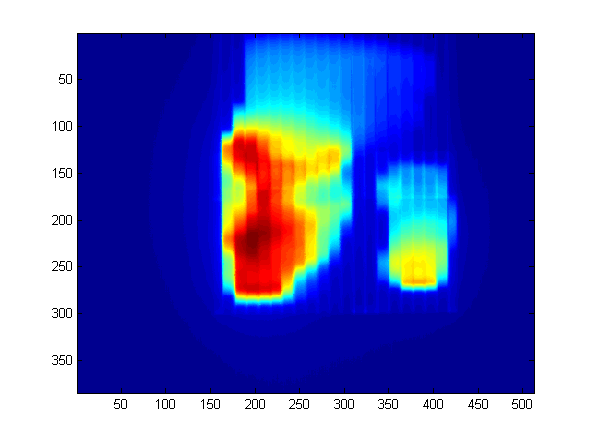
The size of this matrix is 384 px * 512 px, since this is the size of our aS500 imager. The pixel values of the matrix are absolute dose values (expressed in CU - Calibrated Units), because Varian Portal Dosimetry is an absolute method of dose verification. For the David verification, we will ignore this.
Results
Measurement
The deconvoluted David "target" measurement for our 320° sample field looks like this:
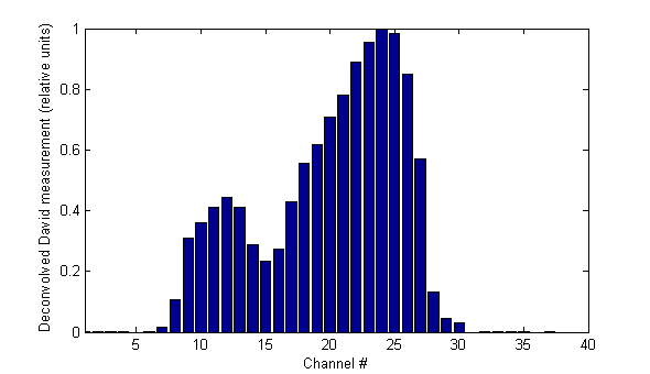
The goal is to predict this measured 1D-distribution by using one of the "candidate" 2D-distributions.
Note: Should you try to match this profile visually with the 2D-distributions shown on this page: you have to take into account that on the 2D-plots the Y1-jaw (the "Target" side if the collimator is at 0°) is on the right. This corresponds to the side of the low channel numbers in the David profiles (channel 1: Target side, channel 40: Gun side). Therefore, the higher peak is right on the 1D-profile, but left on the 2D-plots). Just flip one of them.
The Optimal Fluence Method
For the David prediction, four pixels of the fluence matrix (2.5 mm resolution) were combined laterally to match the 1 cm leaf width.
Since the optimal fluence is the 2D-fluence pattern which is located upstream of the MLC, it should be the "sharpest" of all. This is really the case:
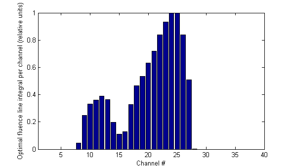
The valley between the two peaks is lower than the measured valley, although the measurement is deconvoluted. The fluence of channel 28 is near zero.
The PDIP Method
Predicting David by PDIP is again a sum over all row values (= line integral), and a lateral combination of 13 pixels which belong to one leaf (the extension of the with from 512 to 520 pixels introduces a very small scale distortion):
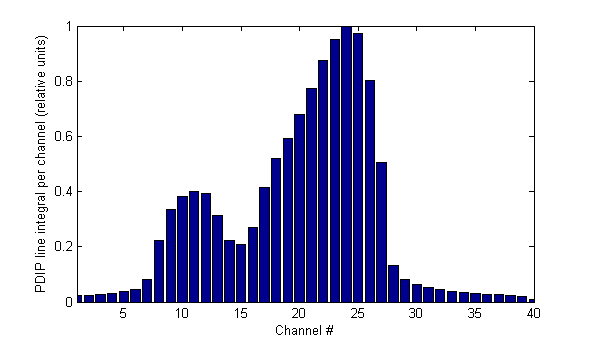
One can see that the big problem of this method is the Physics of the imager (reflected by the PDIP algorithm), which adds long tails on both sides of the field. This is rather disturbing.
Conclusion
Although not necessary for the routine application of the David system, it would be interesting to see that a David 1D-profile can actually be "predicted". This works better for the Optimal Fluence as a source candidate, as for the PDIP matrix.
Unfortunately the most promising candidate, the Actual Fluence, can be visualized, but to our knowledge cannot be exported from the Eclipse TPS. In case we are wrong: any suggestion from Eclipse users is welcome!
Note: the flattening filter (producing the central depression in the 15MV beam) should be no problem for the David prediction: on the TPS side, Eclipse now compensates the beam profile during optimization. On the David side, calibration flattens the measured profile.