Eclipse Calculation Grid - The Unknown Entity
For 20 years or so, the calculation grid size in the TPS played a rather insignificant role in our department. Starting with CadPlan in 1996 and upgrading to Eclipse in June 2002, we knew quite well about the interplay between grid size, calculation time and memory consumption, within the limits defined by hard- and software of the time. Sometimes, during commissioning of a new algorithm, we tested different grid sizes, from the default of 2.5 mm down to the minimum of 1.0 mm, but usually the results were unspectacular, and confirmed the well known rules in this area of tension:
- If you choose a smaller grid, you will wait longer for the results, but isodoses will more closely follow density changes.
- If the grid is too small, you will run into memory problems.
Most importantly, dose was more or less independent on grid, which means that repeating a plan calculation with different grid size and the same MU didn't change dose (simple geometry, no gradient region). Of course there were always small variations within a few tenths of a percent. But since the internals of a TPS are largely unknown to the user anyway, this had to be accepted.
Choosing the default grid size for new plans is always a compromise between speed and accuracy. While for Electrons we use an eMC default grid of 1.5 mm, our Photon default of 2.5 mm was only reduced occasionally, e.g. for stereotactic cases1 or when a higher dose resolution was required for other reasons.
We were suprised to discover that you could end up with 3% dose difference for the PTV, depending on grid, by using the latest algorithms.
The DVH Experiment
In Eclipse, we recalculated clinical SRT plans with different calculation grid settings. Here an example (slice thickness of the patient 3D image is 1 mm):
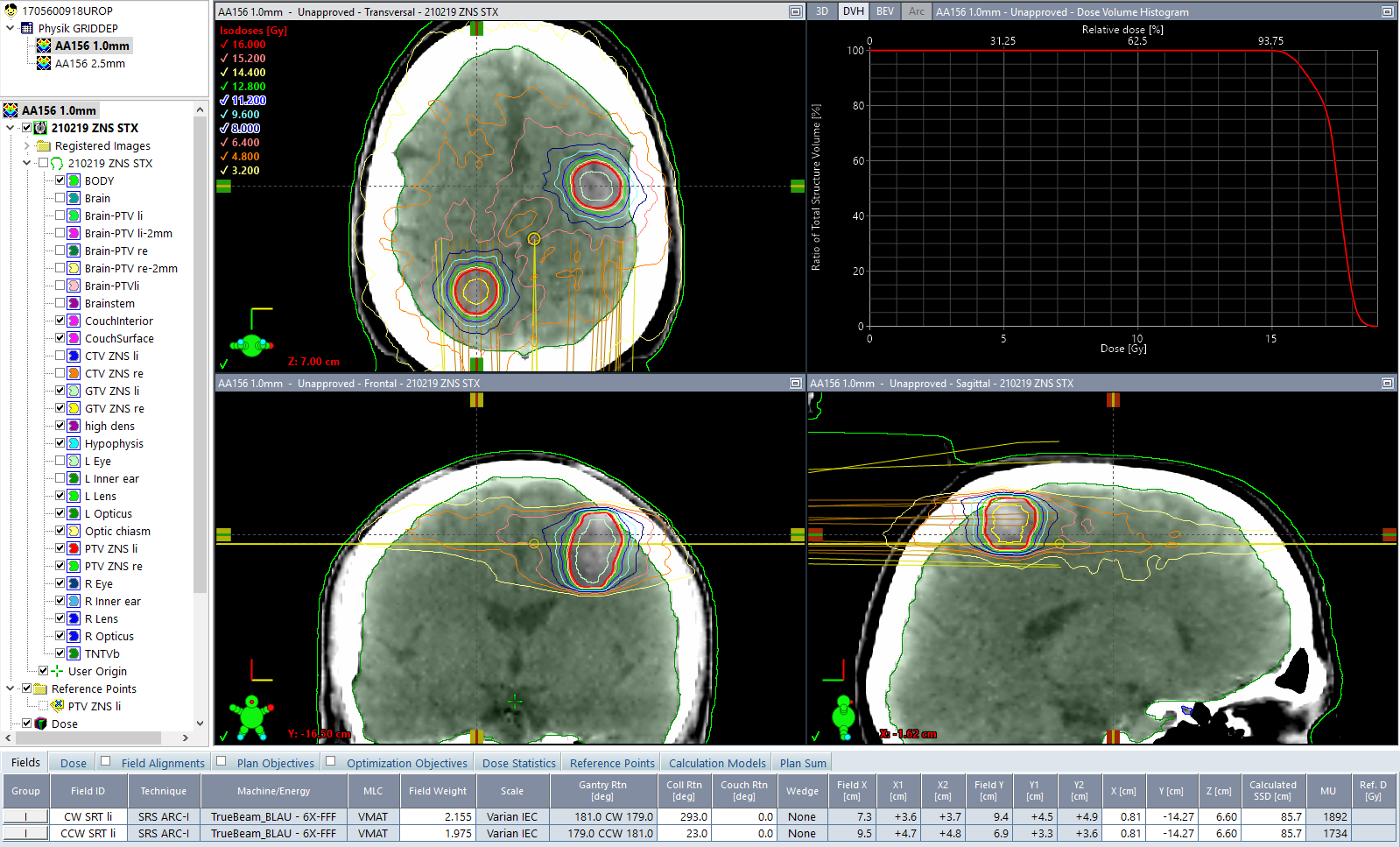
In addition to the clinical plans, we defined simple phantom structure sets with one or two PTVs, and no organs at risk (OAR). To get DVH results for the PTV that could have equally been produced by real patient optimizations, we chose cylindric BODY shapes and spherical PTVs.
In the following image, the BODY is a cylinder with 10 cm diameter. Embedded are the two spheres of 2 cm diameter. The similarity to the brain metastases of the clinical plan is intended:
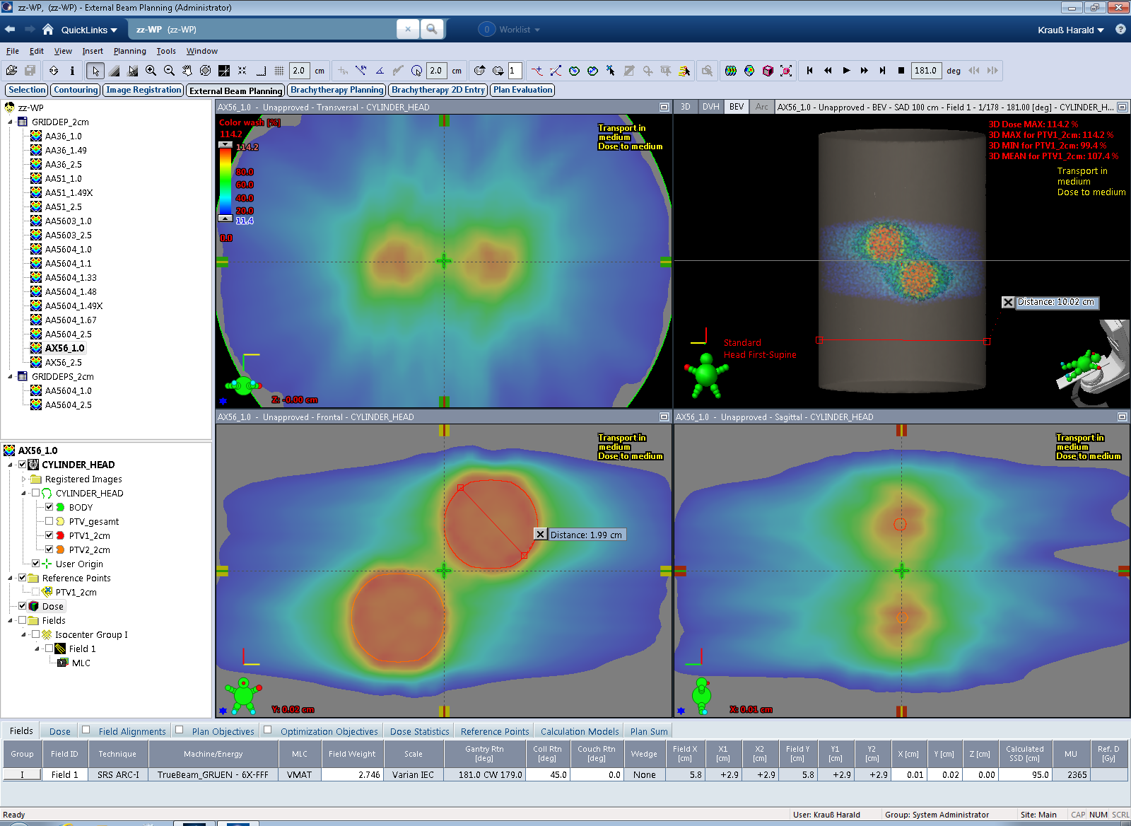
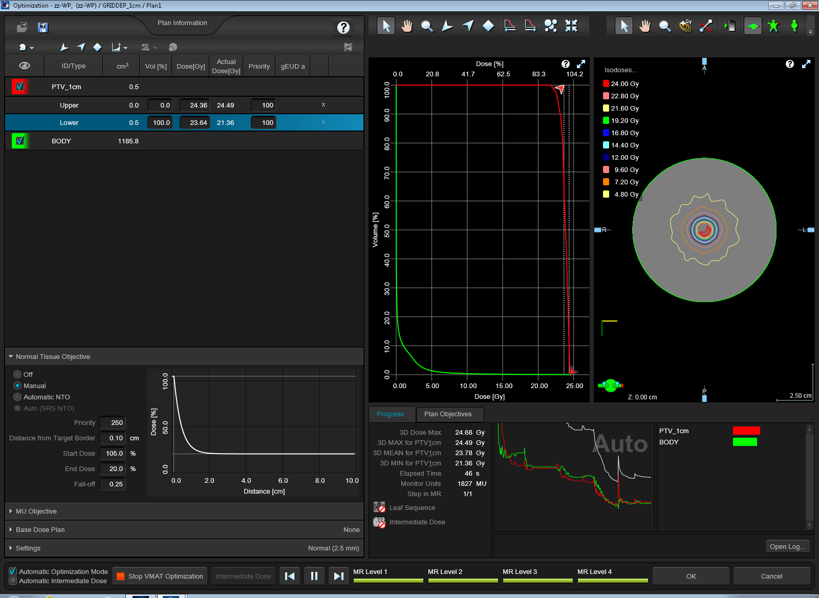
Single Arc VMAT treatments were set up (energy: 6FFF) and the plans (target volume: PTV1) were optimized2 with Photon Optimizer (PO) to give homogeneous dose to both PTVs.
In order to make it not too easy for the optimizer to achieve good results for the PTV(s), and since there were no OARs present in the phantom patient, we "forced" the Normal Tissue Objective (NTO) to counteract in a rather unclinical way: high NTO priority in combination with a requested dose falloff that is impossible to achieve. This will result in PTV-DVHs that will have a shoulder - just like in the clinical plan shown above - rather than a perfect box shape.
Some typical optimization settings are shown in the left part of the image:
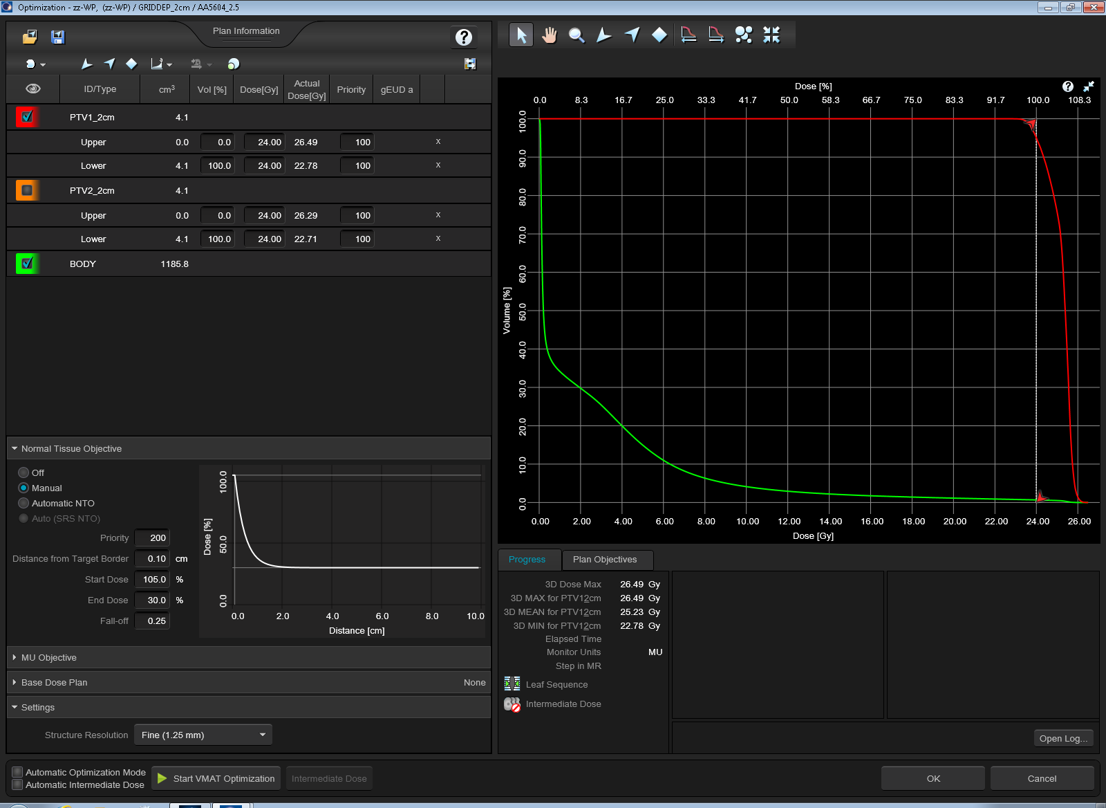
Switching off NTO would instead result in a perfectly box shaped target DVH (red curve),
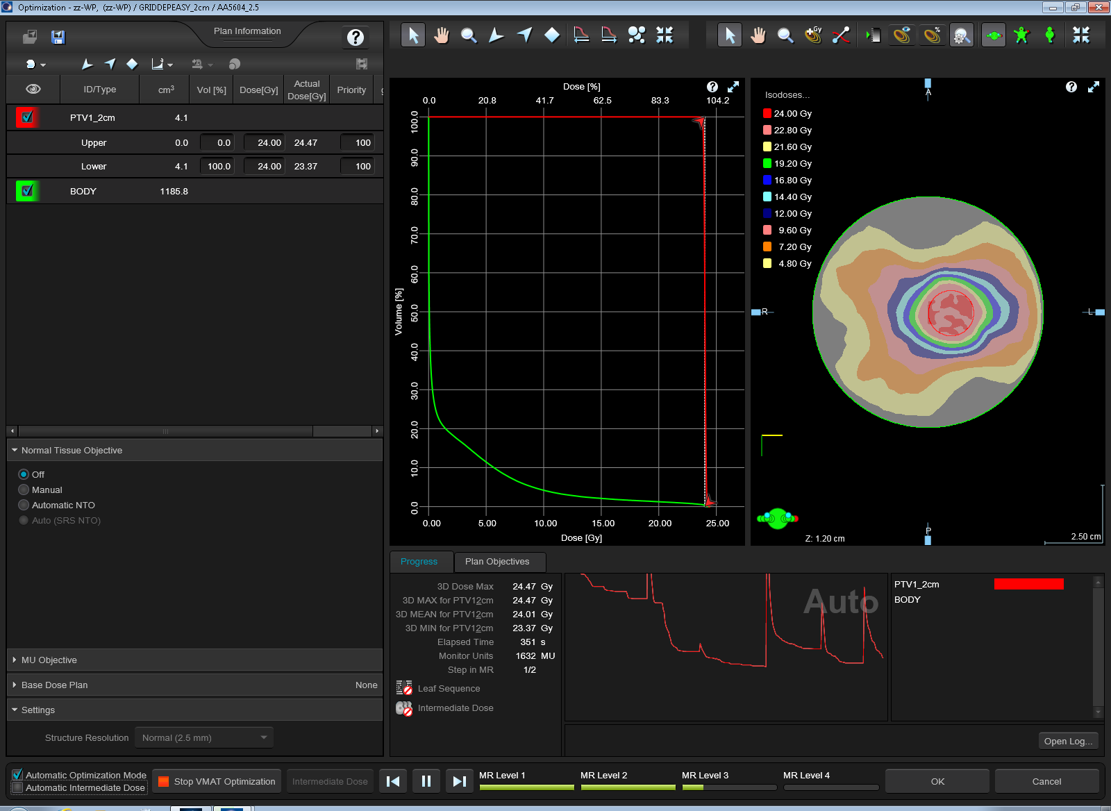
and the compared plans would have very similar mean doses. Therefore it is important for our experiment to keep the strong NTO, which somehow replaces the missing OARs.
3D dose and DVHs were calculated with the standard grid setting first, and then, keeping MU constant, with the alternative grid setting. We declare 2.5 mm being the standard grid and 1.0 mm the alternative grid (although in the clinical plan, the situation was reversed: the stereotactic patient was treated with the 1.0mm-calculated plan). The DVHs for PTV1 in the two calculations were then compared.
Various optimization settings are not relevant for the experiment: whether Structure Resolution is chosen as "Fine" or as "Normal", whether Intermediate Dose is calculated or not (the phantom is filled with water anyway) doesn't have an impact on our plan comparison. Also the Plan Normalization (whether the plan is normalized so that 100% covers 95% of target volume or the plan is normalized to mean dose) doesn't play a role. As long as the MU and the MLC sequence are the same, the two plans, calculated with different grid, can be compared.
We calculated plans and compared DVHs using algorithms AAA 15.6.03 (our clinical default on the live system), AcurosXB (AXB) 15.6.03, AAA 15.1.06, AXB 15.1.06, AAA 13.6.23 and AAA 15.6.04 (the latter two only on TBOX).
One must not make the mistake to compare the results of different algorithms and the same grid. Dose output of different algorithms are allowed to be slightly different, due to independent dose calibration in beam modelling. This is not what interests us here. Here, we only want to see how calculated dose depends on grid, within the same algorithm.
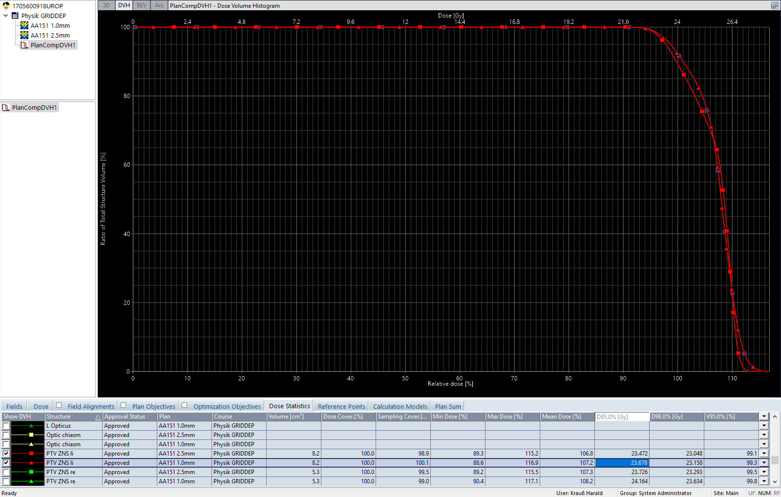
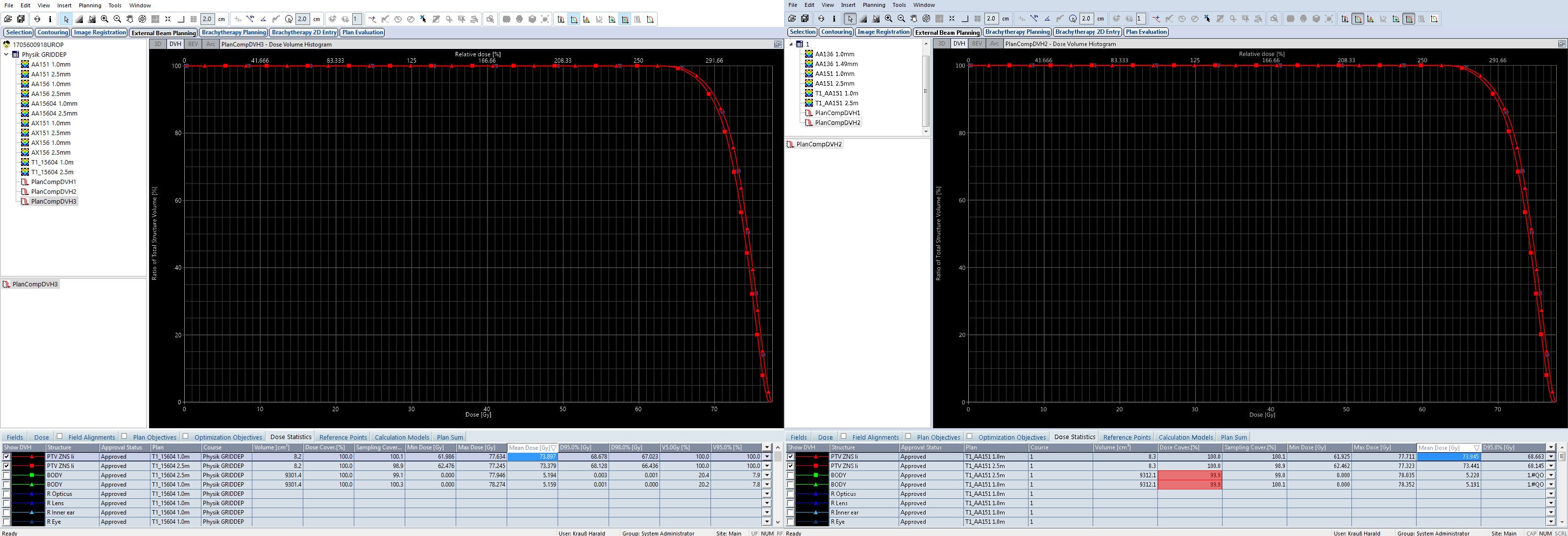
Surprising Results - AAA
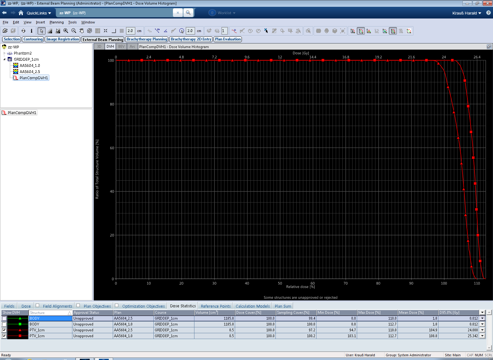
When calculated with AAA 15.6.03 and 1.0 mm grid, the clinical plan shows higher dose to the PTVs (the DVH curve seems to be shifted to the right) compared to the calculation with 2.5 mm grid. For the larger of the two targets (volume: 8.2 ccm), shown in red, the mean dose in the 1.0 mm calculation is 2.6% higher. However, the treated plan was not normalized to target mean, but to D95% (prescription dose was 24 Gy in 3 fractions). If we use this metric3, the 2.5 mm calculated plan has a D95% dose of 23.253 Gy instead of 24.000 Gy, which is 0.75 Gy less, for the same number of Monitor Units. This corresponds to a dose difference of 3.1%:

Dose is consistently higher throughout the whole DVH, and the curves never cross. One may object that a grid of 2.5 mm is simply not appropriate for target structures of 5 to 8 ccm volume. Granted. The result is nevertheless unusual and triggers the question: "Which one is correct?"
Let's look at older versions of AAA. We copy the plan (preserving MU), and recalculate both versions with AAA 15.1.06:
The difference in mean dose to the red PTV is much smaller (0.4%) compared to the 2.6% of AAA 15.6.03.
The green PTV is smaller in size (5.2 ccm) than the red one. The difference in mean dose for the two grid sizes is 2.9% (AAA15.6.03) and 0.9% (AAA15.1.06). See the Dose Statistcs tab.
For the even older AAA, 13.6.23, we will have to switch to the TBOX (on the live system, 13.6 has already been removed). But first we stay on the live system and look at the Acuros results.
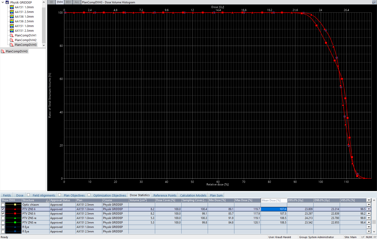
Surprising Results - also for Acuros XB
The first screenshot shows the two curves for AXB 15.6.03, the red PTV. Triangles are for 1.0 mm, squares for 2.5 mm. Results are similar to AAA 15.6.03. At 95% volume (where the clinical plan hadd been normalized), the dose difference (1.045 Gy) is even larger than for AAA, but the difference in mean dose (2.4%) is a little less. The curves are simply not parallel, so it makes a difference where they are evaluated.

The older AXB 15.1.06 however produces DVH curves that are much closer to each other. Difference in mean dose is only 0.1% for the red PTV:
The following table sums up the results for the live system calculations performed on the patient data set:
| Patient data, PTV "red" | Dmean, Grid 2.5 mm [%] | Dmean, Grid 1.0 mm [%] | Delta [%] |
|---|---|---|---|
| AAA 15.6.03 | 105.9 | 108.5 | 2.6 |
| Acuros XB 15.6.03 | 106.5 | 108.9 | 2.4 |
| AAA 15.1.06 | 106.8 | 107.2 | 0.4 |
| Acuros XB 15.1.06 | 107.5 | 107.6 | 0.1 |
The overall picture is the same for AAA and for AXB: the finer grid results in higher mean doses, if the 15.6 version is used.
More Tests on the TBOX
Looking for 13.6 results is also the opportunity to switch to a phantom instead of a real patient. As we have seen for the two PTVs (red and green), dose difference between the two grids seems to depend on the size of the targets too. Therefore, we generate phantoms with pairs4 of spherical targets (diameters: 2 cm and 5 cm). The slice thickness of the phantom is again 1 mm, as in the patient data set.
The following tables sum up the findings for the phantom with the spheres. Since both spheres in a phantom have the same size, we only report the results for PTV1.
The TBOX runs Eclipse 15.6 MR1, and this "Maintenance Release 1" introduced the new algorithm version 15.6.04 (with the exception of AAA, the difference is only in the version number).
| PTV Size: 2 cm | Dmean, Grid 2.5 mm [%] | Dmean, Grid 1.0 mm [%] | Delta [%] |
|---|---|---|---|
| AAA 15.6.04 | 105.1 | 107.2 | 2.1 |
| Acuros XB 15.6.03 | 105.5 | 107.4 | 1.9 |
| AAA 15.1.06 | 106.0 | 106.2 | 0.2 |
| Acuros XB 15.1.06 | 106.3 | 106.4 | 0.1 |
| AAA 13.6.23 | 106.0 | 106.2 | 0.2 |
| Acuros XB 13.6.23 | 106.2 | 106.2 | 0.0 |
Remember that the mean doses in % should not be compared across algorithms, because there are other reasons why they can be different.
The next table shows the results for larger PTVs (spheres of 5 cm diameter):
| PTV Size: 5 cm | Dmean, Grid 2.5 mm [%] | Dmean, Grid 1.0 mm [%] | Delta [%] |
|---|---|---|---|
| AAA 15.6.04 | 107.2 | 108.2 | 1.0 |
| Acuros XB 15.6.03 | 106.9 | 107.5 | 0.6 |
| AAA 15.1.06 | 107.8 | 108.1 | 0.3 |
| Acuros XB 15.1.06 | 107.4 | 107.5 | 0.1 |
| AAA 13.6.23 | 107.8 | 108.2 | 0.4 |
| Acuros XB 13.6.23 | 107.2 | 107.4 | 0.2 |
Also for the larger 5 cm target, the 15.6 versions have the largest dose difference between the two grid sizes. However, the effect is less pronounced.
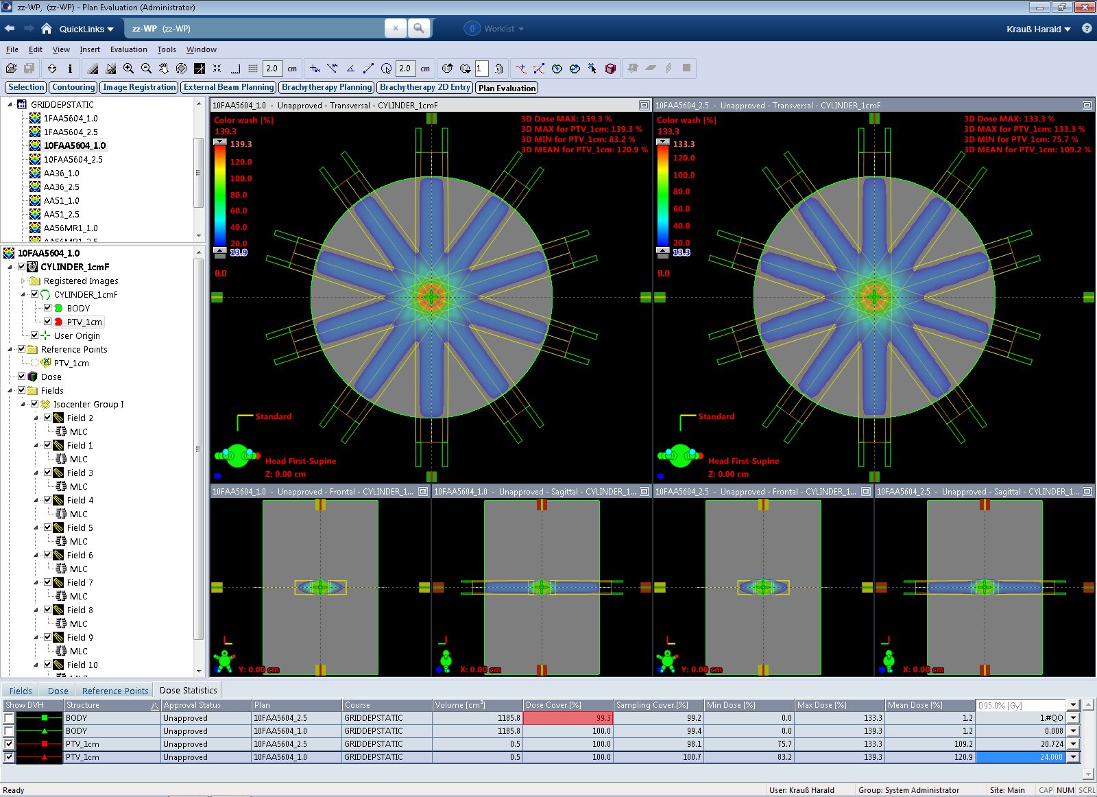
As a final challenge, we optimize to a single, spherical target of 1 cm diameter:

Again, the strong NTO counteracts the PTV:
The DVH comparison for AAA 15.6.04 is not quite what we wanted to see, but the result could be expected:
Difference in mean dose is 3.9%. Considering the fact that on a 2.5 mm grid there are no more than four dose sampling points across a 1 cm sphere, it is clear that the reported mean doses are not expected to be equal for the two grids. However, the figures for AAA 15.6 and AXB 15.6 and the 2.5 mm grid are a little low, which could be the reason for the larger 15.6 deltas:
| PTV Size: 1 cm | Dmean, Grid 2.5 mm [%] | Dmean, Grid 1.0 mm [%] | Delta [%] |
|---|---|---|---|
| AAA 15.6.04 | 104.9 | 108.8 | 3.9 |
| Acuros XB 15.6.03 | 105.2 | 109.5 | 4.3 |
| AAA 15.1.06 | 105.8 | 107.9 | 2.1 |
| Acuros XB 15.1.06 | 106.0 | 108.7 | 2.7 |
| AAA 13.6.23 | 105.9 | 107.9 | 2.0 |
| Acuros XB 13.6.23 | 105.9 | 108.6 | 2.7 |
It is often helpful to strip down the problem to simple cases. If we move away from VMAT and DVHs, the most direct approach is to compare static fields calculated with different grid settings,
and finally single PDDs:

It turns out that the differences already start here.
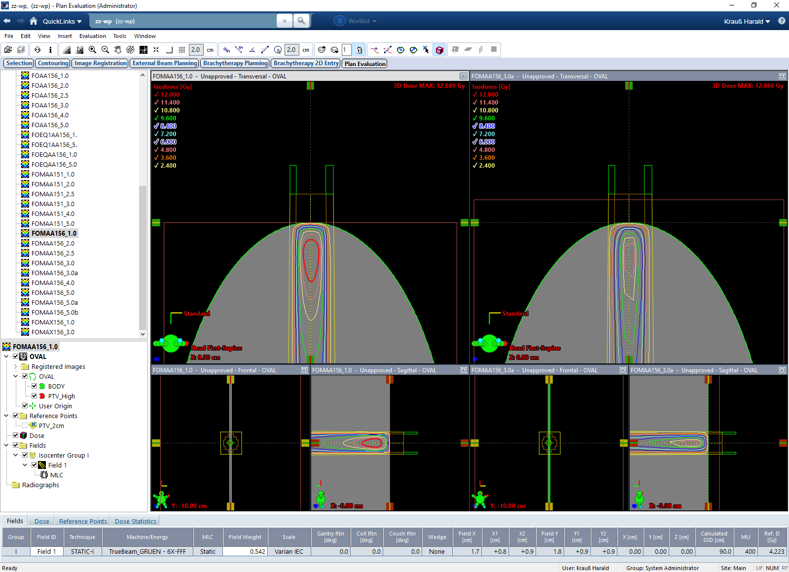
Static Fields
We switch the technique from "SRS STATIC" to "STATIC". This way, we can calculate with grids up to 5 mm (with AAA), which will be instructive.
The simplified setup is an oval shaped phantom and a static isocentric MLC field (HD120 MLC with 2.5 mm leaf width). A PTV of 1 cm diameter is also contained, but we will only compare depth dose curves in the center of the field.
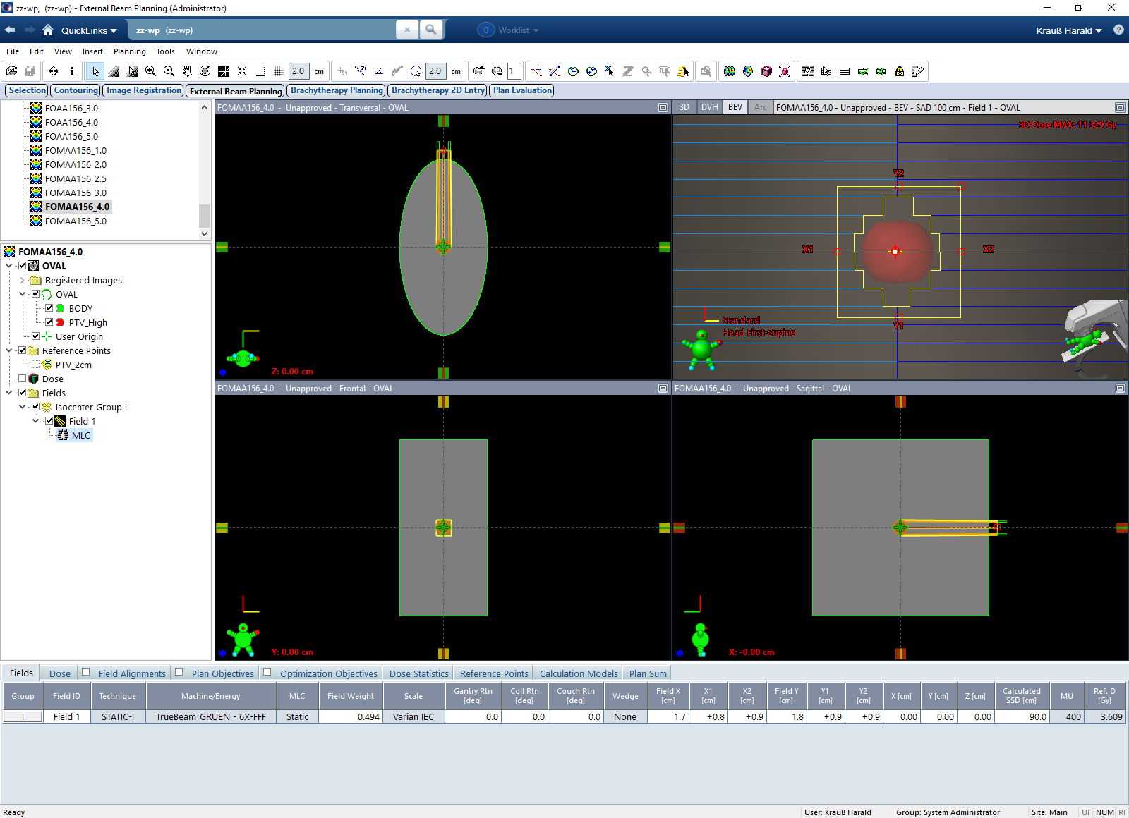
All plans are identical copies, the only difference is in the grid.
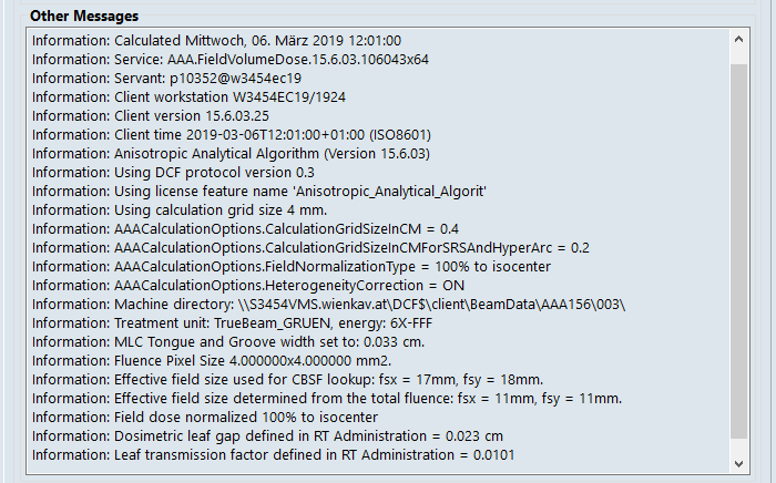
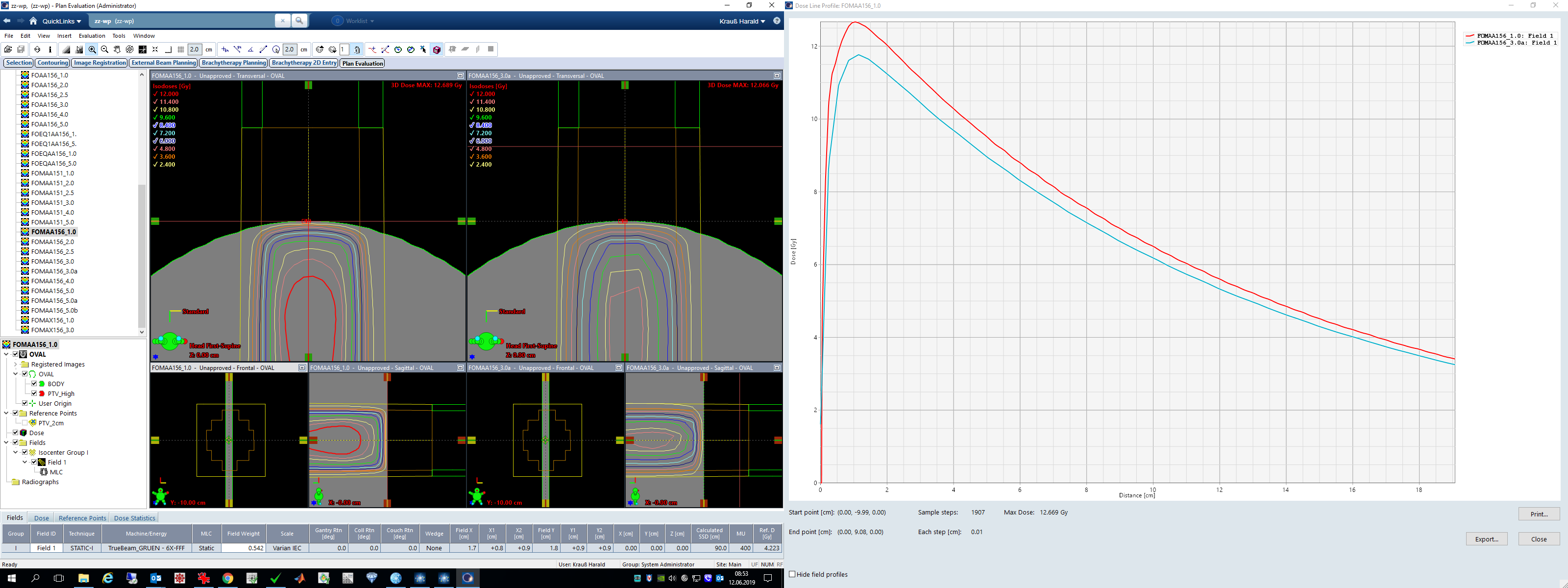
In the following sequence of AAA plan comparisons, the 1 mm plan is the left plan (red PDD). The comparison plan to the right has a grid of 2.0, 2.5, 3.0, 4.0 and 5.0 mm (PDD in cyan).
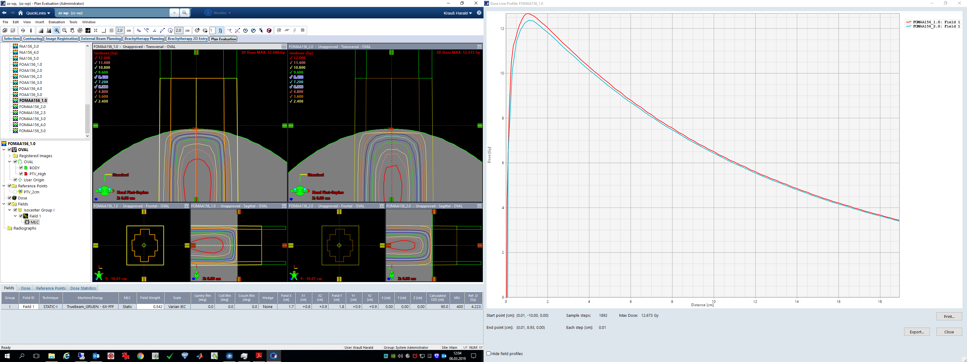
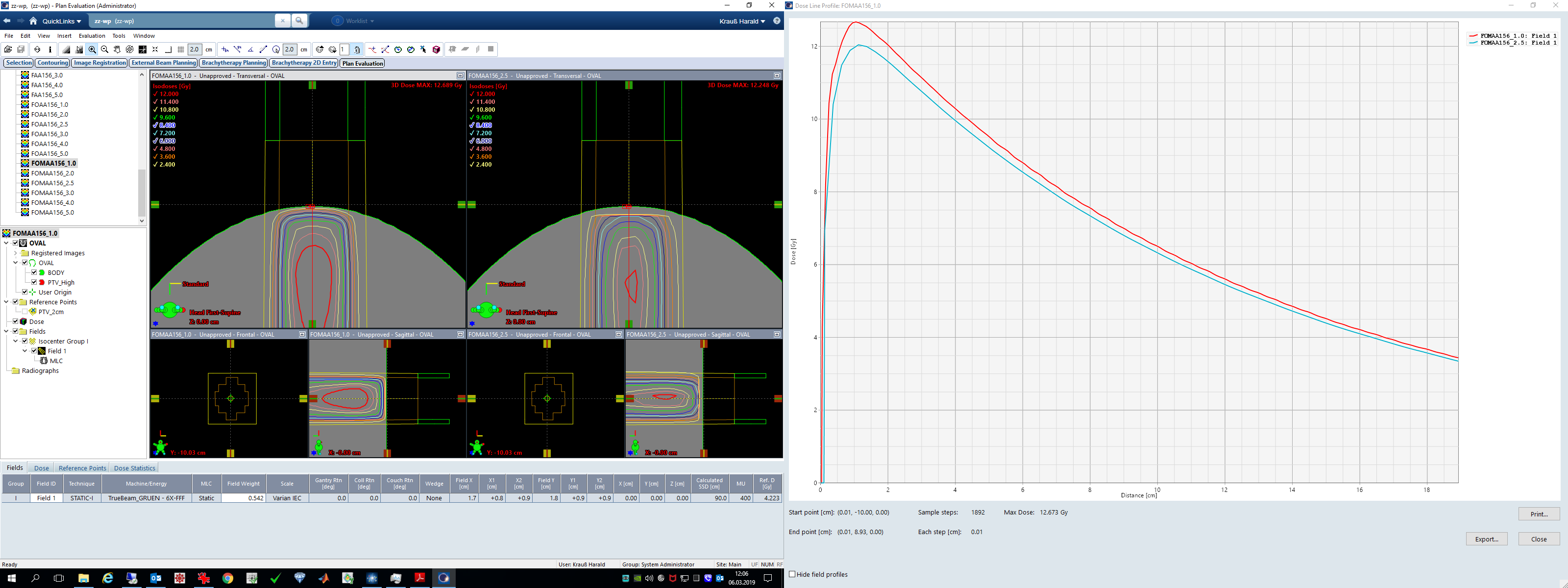

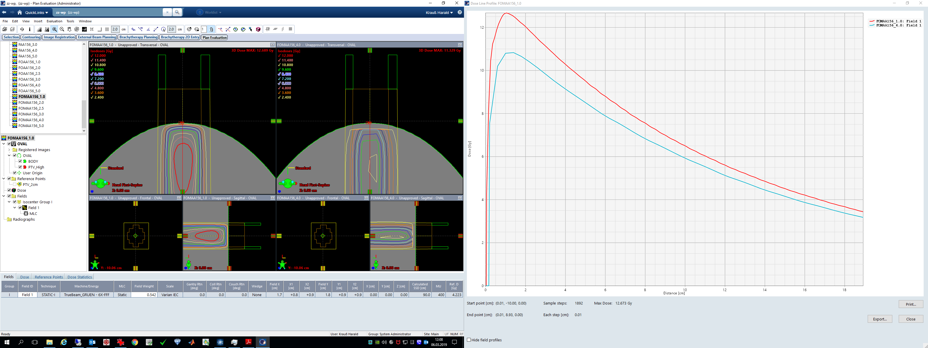
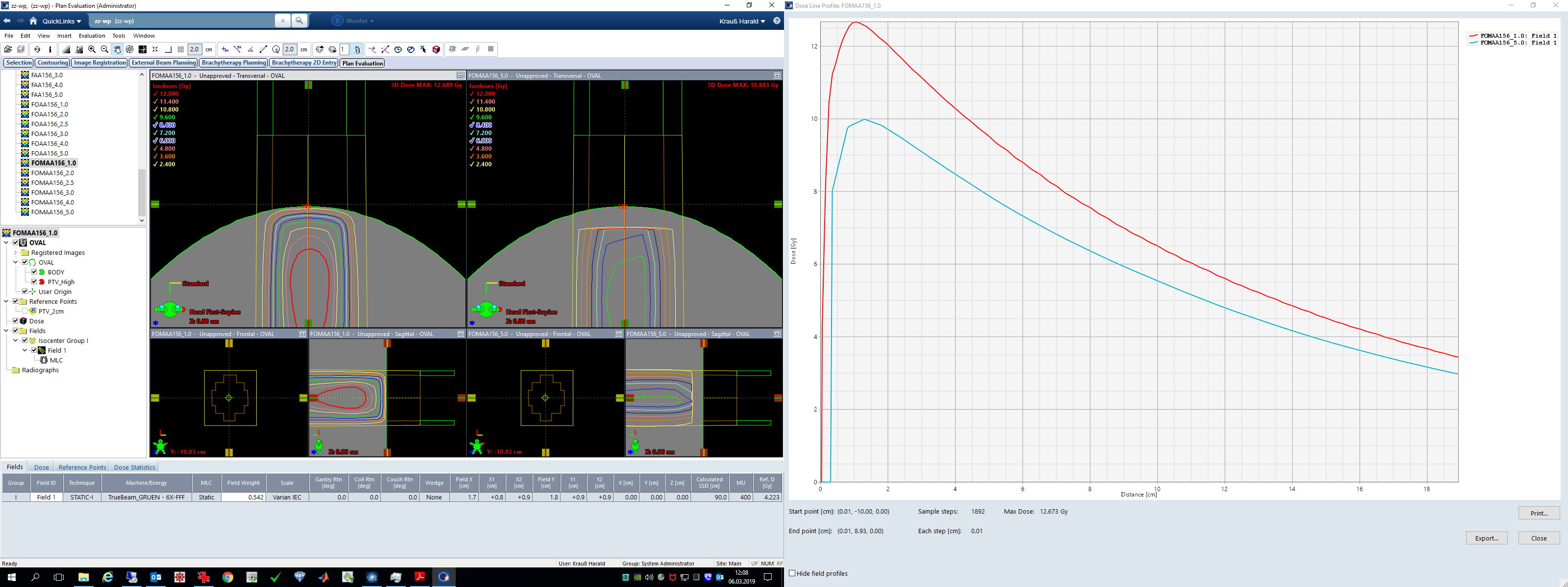
As grid gets coarser, less and less dose is delivered through the small MLC opening of constant size. One could argue that a grid of 3 or 5 mm is way too large for such a small field size. However, during VMAT, small openings are very common, and the user cannot control them.
The first sentence in Chapter 12 of the Algorithms Reference Guide is this:
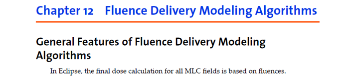
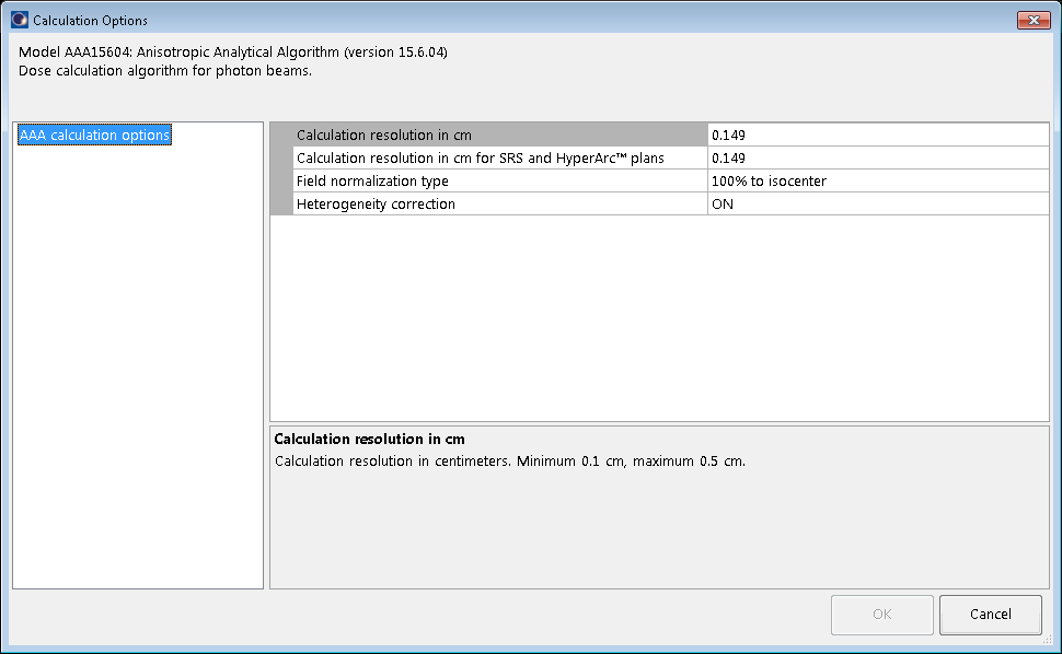
Indeed, when we open the Dose Calculation Log in Field Properties, we find that the Fluence Pixel Size is 4.0 x 4.0 mm2 for a calculation grid of 0.4 cm:
This doesn't explain the observed differences between the 15.6 and older releases, because in all investigated versions of AAA, fluence pixel size equals grid size (for AXB, fluence pixel size is always half the grid size).
But it may explain, besides the other conceptual differences between Acuros and AAA, why Acuros performs better for small fields: fluence grid is always twice as fine as for AAA. This can be demonstrated if we compare the 1 mm and 3 mm calculations of the static MLC field for AAA and AXB.
For AAA 15.6, the dose difference between 1.0 mm and 3.0 mm grid in dmax is 0.9 Gy or 7%:
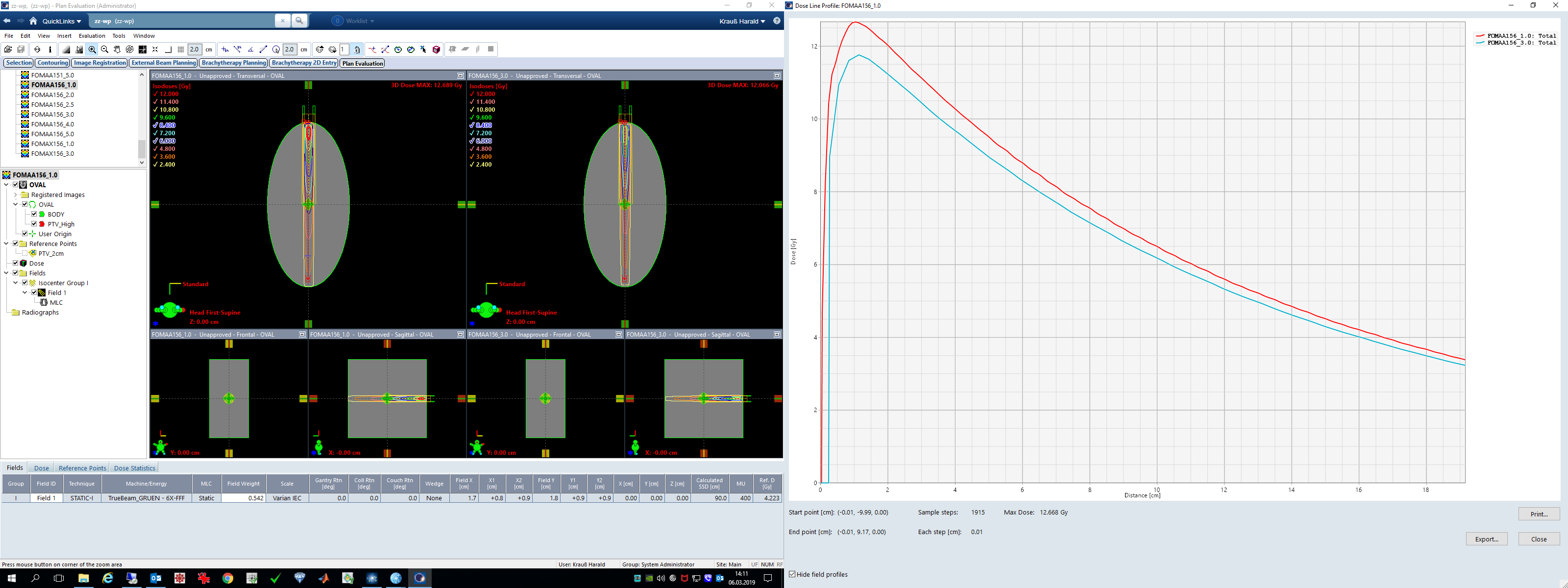
For AXB 15.6, the same difference is only 0.18 Gy or 1.5%:
So far, there is no conclusion. The case is still open. Maybe we missed an important point, so we wait for a statement from Varian engineering (see response from Varian at the bottom of the page).
More Open Questions ...
In our DVH experiment, we have compared calculations that use two different grids: 1.0 mm and 2.5 mm. Intermediate grids gave intermediate results, so we didn't report them (except for a special case - see below).
For a given (small) target size, why is grid dependence larger in the 15.6 versions? Or is the whole thing an artefact produced by the rather "special" geometry?
Generally speaking, it is difficult if not impossible for the user to verify that a DVH is calculated correctly by the TPS. The user can only perform plausibility checks and compare with older versions. However, the dose differences are too small for a plausibility check to fail, and the question which DVH is the correct one, remains open.
The "Grid of Death"
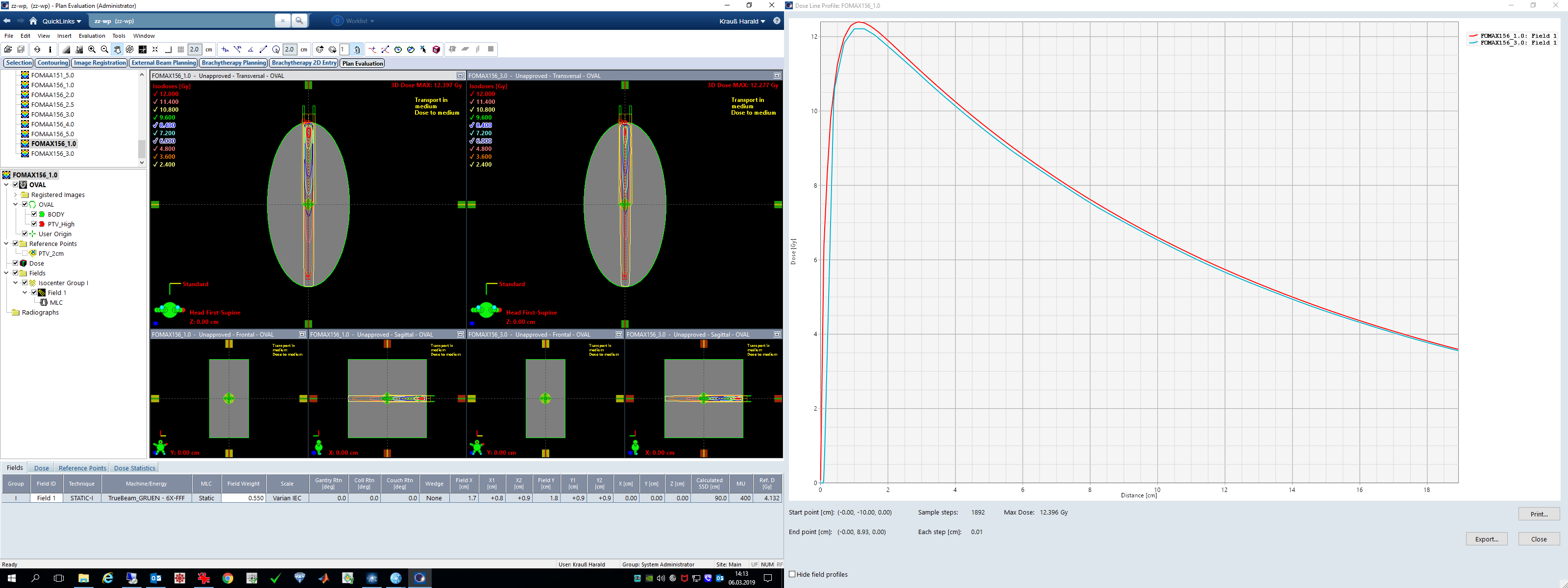
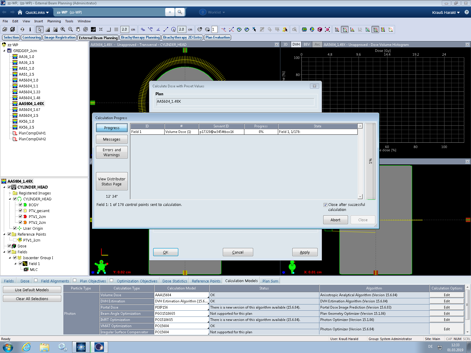
Ever tried to calculate using odd grid sizes such as 1.33 mm or 1.67 mm? Probably not. We don't even know how Eclipse processes input if the user chooses to enter such numbers in the Calculation Options. Anyway, we found out that entering 0.149 cm will have a strange consequence.
If we enter this number and try to calculate dose, nothing will happen. All progress bars will remain in their initial configuration, forever. Here the progress on the live system running 15.6 (AAA 15.6.03) after 20 minutes:
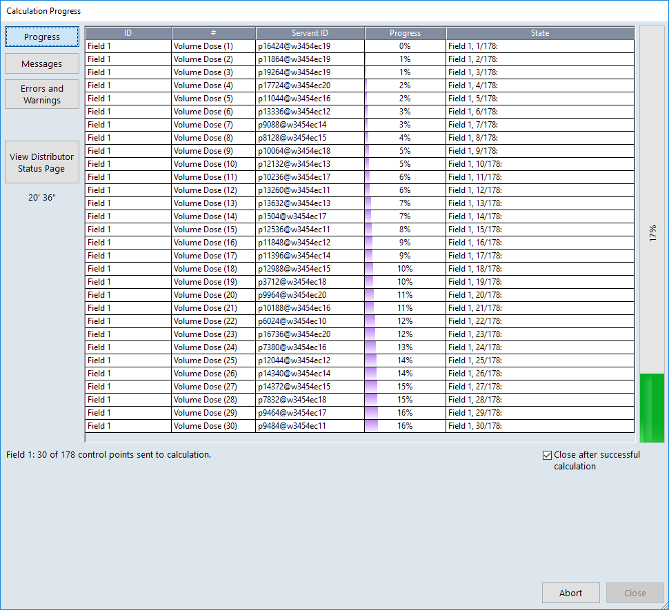
... and after 33 minutes. No errors, no warnings, no progress:

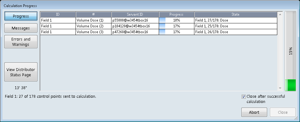
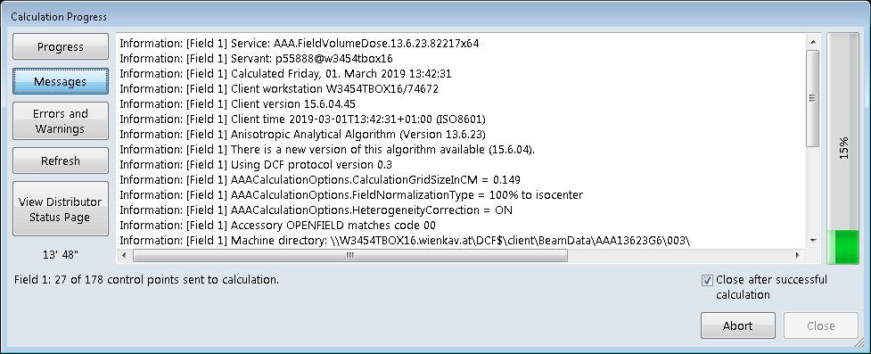
Here the same on our TBOX running the (currently) latest release, Eclipse 15.6 MR1 (AAA 15.6.04), with Control point field parallelization temporarily turned Off (only one progress bar):
You can wait indefinitely, or press the Abort button (and do some cleanup). We call this the Grid of Death (GOD).
Keep in mind that if you work in a DCF with several agents, the use of GOD will cause data traffic congestion. Depending on the number of agents, "Calls waiting" may build up rapidly. So if you want to tease your co-workers a little bit ...
Version note: death strikes only for version 15.1 and higher. Interestingly, the older AAA 13.6.23 accepts the odd grid size of 0.149 cm and starts calculating:
Response from Varian
Here is the statement from Varian engineering (2019-05-06):
"Investigation Conclusion: The main title for the complaint was "Customer noticed a rather strong dose dependence on calculation grid size for AAA 15.6. It is larger than in previous versions of AAA (15.1)." After investigating the complaint it was shown that the main difference between 15.1 and 15.6 is the increase of accuracy in the modelling of the tongue and groove, TNG, of the Multi Leaf Collimator, MLC. This effect is more noticeable in higher resolutions ~1mm as the TNG is small. After comparing the profiles of both 15.1 and 15.6 on multiple patients it was shown that 1mm resolution more accurately models the dose in the patient and also has an overall increase in energy in the peak areas. Conversely the 2.5mm resolution is barely changed. The combination leads a separation in the accuracy of the Algorithm versions, due to a more accurately modeled result for higher resolution.
The complaint also provided a PDF from the client showcasing other issues which were also investigated. The customer named "Grid of death" was tested and a fix implemented in the latest version.
The static field investigation highlights the issue of trying to resolve a small field with too low resolution (>2.5mm). VMAT uses small fields and as such should be highly resolved. That is the same for small static fields or indeed IMRT.
The last effect studied was the effect observed in static3.png, it appears as the grid resolution gets larger the profile shifts inwards. This is most likely due to an overly tight constraint on the calculation volume used in the plan.
The conclusion of this investigation is to say that small fields should use higher resolutions and that the main differences in versions is due to an increase in accuracy in the higher resolutions."
Regarding the tongue and groove explanation of the differences, we probably have to believe it without being able to verify. At least we can set leaf transmission to 1 (which will, by rendering the MLC "transparent", not only eliminate tongue and groove but the entire MLC) and check whether this has an impact on grid dependence.
Indeed, a transparent MLC will eliminate version differences (left: AAA 15.6.04, right: AAA 15.1):
Since we cannot switch on and off tongue and groove separately, it is questionable whether this is a sensitive test. However, if we would still see version differences here, they would probably have other sources.
As we didn't understand the term "overly tight constraint on the calculation volume" when the Varian engineers talked about static field behavior, we asked for a clarification. We got the following response:
"To clarify the last point, if the user tries to reduce the volume used in the calculation and has it set so that it is inside the body/phantom, then this can result in the issue referenced.
It is set so that as you increase the calculation resolution the calculation volume readjusts slightly so that it takes into account the start of the body. If the calculation volume is set to start inside the body, then this cannot happen and results in what appears to be a half voxel shift.
This was the only way in which I could reproduce the results shown in static3.png (included above, also yes this is referring to the website and the report that they sent. So to say “tight constraint”, too tight or undersized calculation volume was meant.
In summary, to avoid this in future please make sure that the calculation volume is clearly set to be outside the body/phantom."
The screenshot they referred to ("static3.png") and which they included in the mail was actually static5.png, which is shown once again:
However, they didn't get our point. We were not focussing on the isodoses in the plan on the right (which are obviously cut due to the calculation volume set too small), but on the missing dose along the whole PDD.
Firstly, we never set the calculation volume by hand. We assume that Eclipse takes care of that, so that when a plan is generated, the calculation volume is adjusted automatically to cover whole body.
Secondly, even if we decide to adjust the calculation volume manually, dose inside does not change. Here the same pair of plans, with the calculation volume on the right generously enlarged:
Isodoses are not cut anymore, but dose at dmax (and beyond dmax) is still at the same low level in the 3 mm plan as before.
Here once more the comparison including PDDs:
The overall dose discrepancy does not change. So we still don't have a satisfying explanation of this effect.
Notes
1 Starting with Eclipse 15.5, the calculation options offer two grid settings, one for "normal" plans and one for "SRS or HyperArc" plans. We see no benefit in this grid splitting. Eclipse forces the user to use the technique "SRS STATIC" or "SRS ARC", if MU are above a certain limit (1499 for VMAT). This is a too simple rule to automatically differentiate between normal and SRS treatments, as the clinician defines them. Typical palliative spine treatments (single VMAT arc of 8 Gy, requiring 2300 MU or more) treat large PTVs, and clinically do neither require stereotactic accuracy nor a finer grid. But because the plan is above the MU limit for normal arcs, it has to be calculated with the technique changed to "SRS ARC", and therefore the SRS grid will be used. Starting with 15.5, the user must always be aware of the normal/SRS technique status of the plan. If the default SRS grid is smaller than the normal grid (which is probably Varian's idea), this can lead to longer calculation times (and an unnecessarily high dose resolution) with the user not even knowing that he/she is calculating SRS. The only solution is to use the SAME default grid for both techniques, which renders the whole idea of grid splitting superfluous.
2 The optimization for the phantom, just as the optimization for the example patient, were only performed once. All other plans were copies of the original plan, preserving MU, and only changing algorithm and grid.
3 To keep things simple, we will from now focus on relative mean doses (in percent).
4 Don't get confused why all PTVs appear in "pairs". The effect can be demonstrated with single targets as well, see the 1 cm example.