ISC plans have the same complexity as IMRT plans, which makes it nearly impossible to perform an independent Monitor Unit calculation. Our QA policy is to verify the treatment plan by measuring absolute dose, field by field. For this task, either the 2D-ARRAY or Portal Dosimetry can used. The latter is the most uncomplicated and quick way to verify IMRT dose.The former is more accurate. With the 2D-ARRAY, verifying a complete plan on the linac takes no more than 15-20 minutes, including setup and Array warmup. With Portal Dosimetry, it is even less.
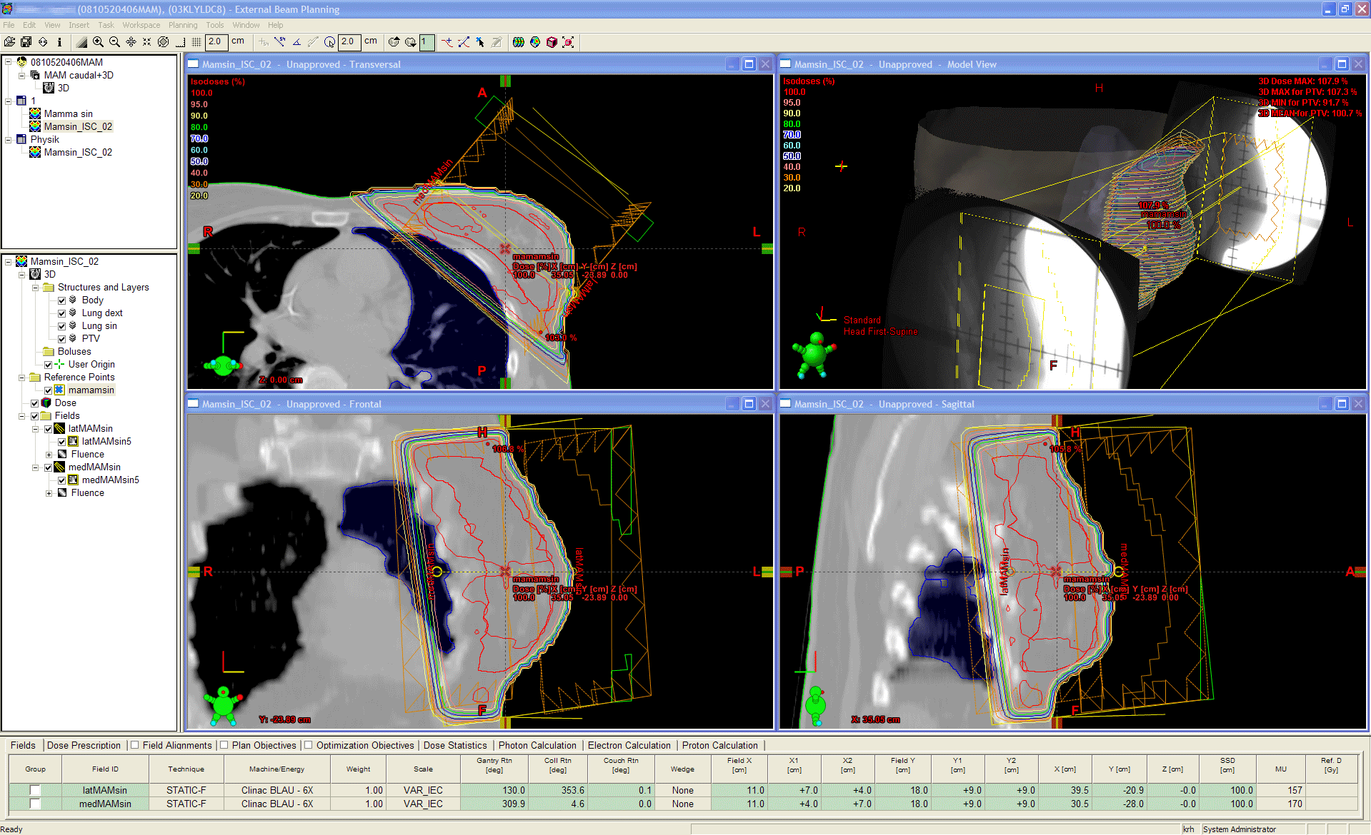
Let's say this is the clinical plan which shall be verified with the 2D-ARRAY:
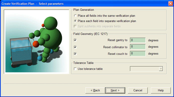
The first step is to prepare the verification plans in Eclipse. This is done by selecting the plan to verify and choose "Create verification plan ..." from the menu. This copies the plan to a CT-scanned phantom on a field-by-field-basis.
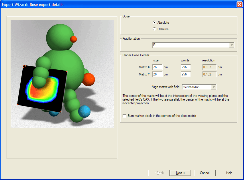
The next step is to calculate dose of both verification plans. The coronal dose plane in depth of the effective point of measurement "Planned Dose File" is exported as DICOM-file in absolute dose units.
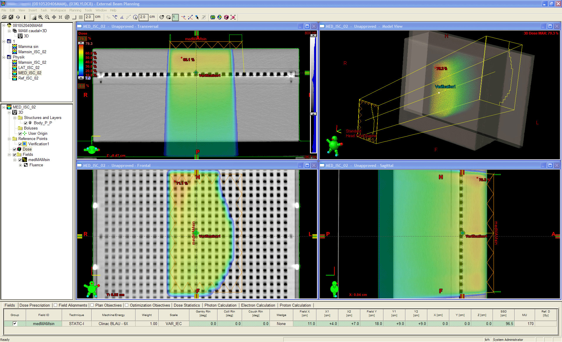
The size of the plane is chosen to cover at least the full treatment field, but this is not critical. Also the resolution of the dose matrix is not critical, as long as it is well below the resolution of the 2D-ARRAY (VeriSoft will later interpolate the lower resolution distribution - the measurement - to the higher resolution distribution - the dose plane).
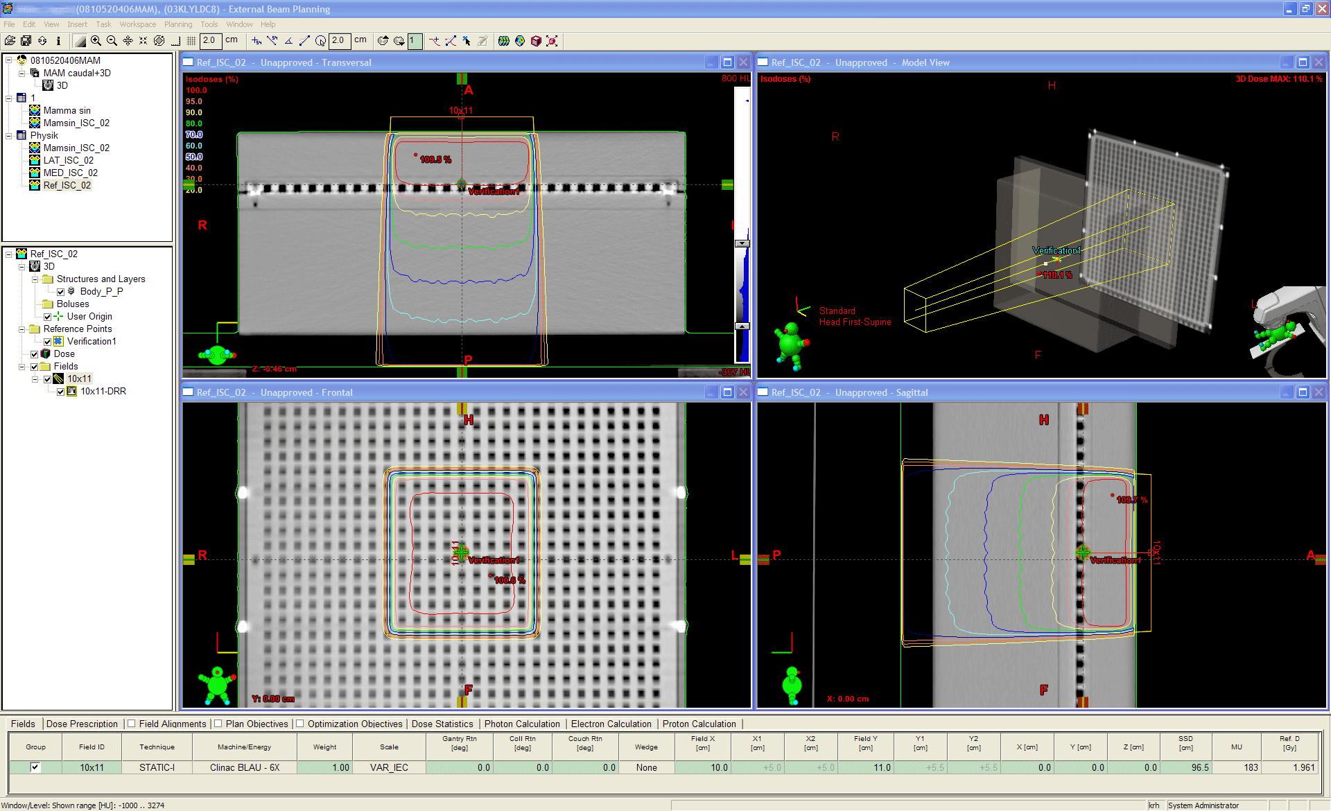
In order to get rid of small calibration deviations of the linac, small inaccuracies during setup, small temperature and pressure misreadings, small HU inaccuracies etc., we copy one of the Verification Plans and paste it as Reference Plan. This gives the plan exactly the same isocenter as the Verification Plans. The fluence is deleted, the field size set to X=10cm and Y=11cm (why 11? see below). This plan is a conventional static plan. Dose is calculated, normalized to, e.g., 2Gy at isocenter (again, this is not critical, as long as it is absolute dose. One could as well calculate a FixedMU plan) and the coronal dose plane in depth of the effective point of measurement is exported as above. Taking this plan as reference means "believing that it is correctly calculated in the TPS".
At last, one has to decide how the plan shall be delivered on the linac. Delivery can either be done automatically via ARIA or manually in Clinac Service Mode. If ARIA is chosen, one has to create an appointment in Time Planner. After the patient is checked in, she appears on the linac's Queue and can be loaded.
If one choses Service Mode for more flexibility (e.g., to repeat a measurement several times without fuzzing around with the verification system), a little more manual preparation is necessary: the dynamic MLC-files have to be exported so that they can later be loaded on the linac with MLC Software. This completes the preparation in the TPS. The files at this stage are organized in the following way:
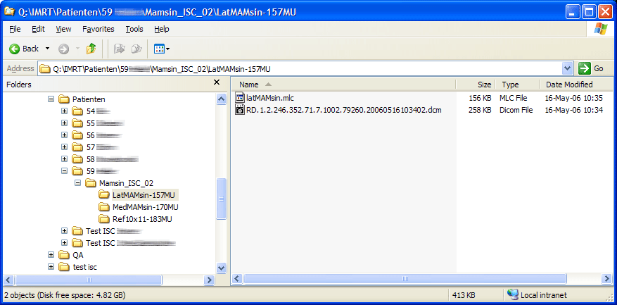
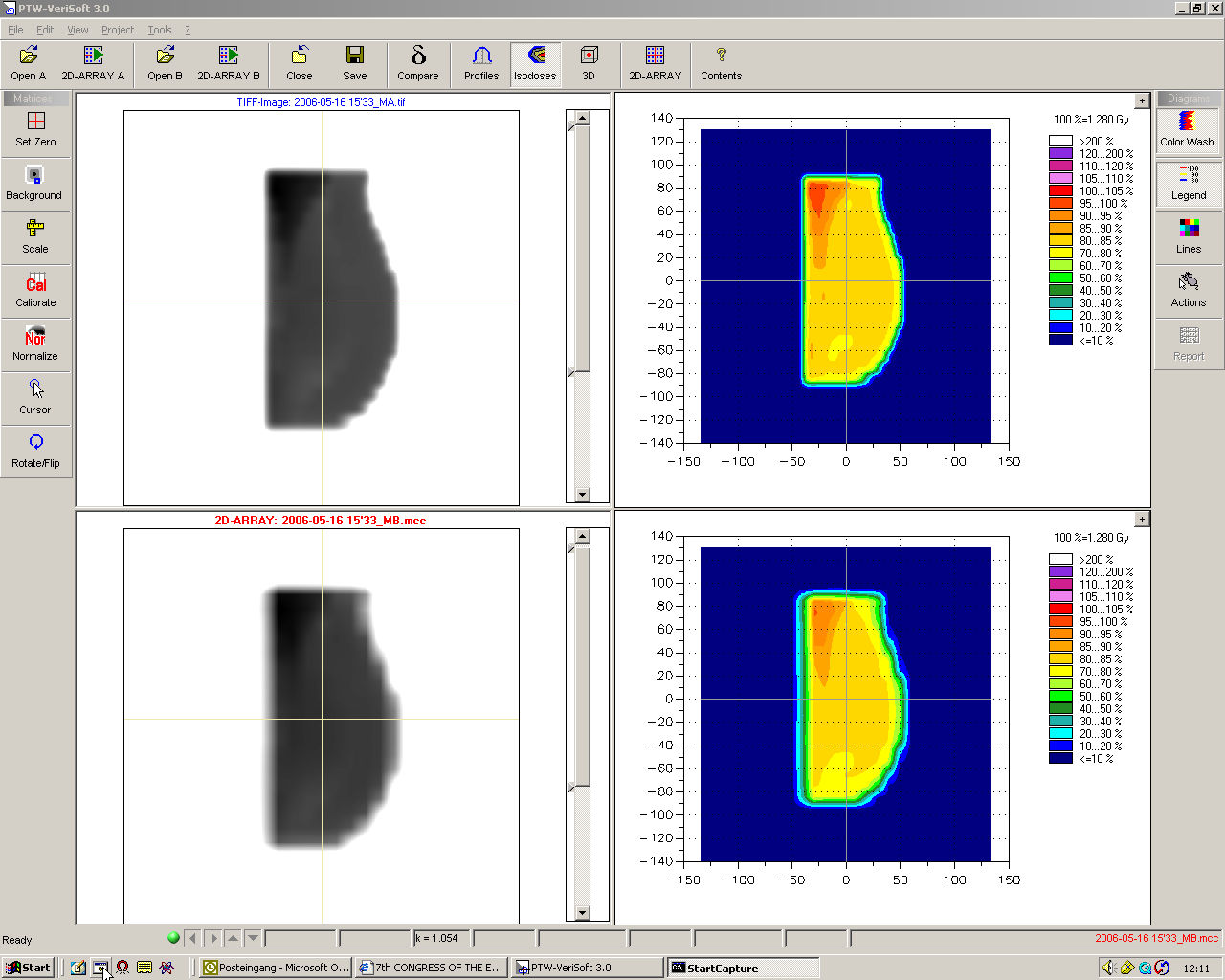
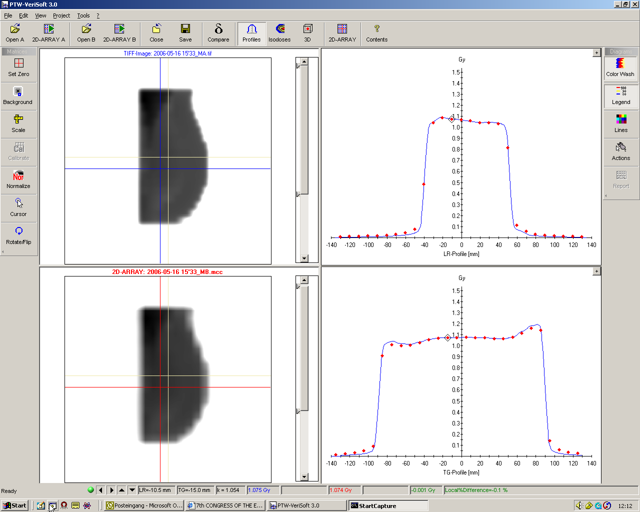
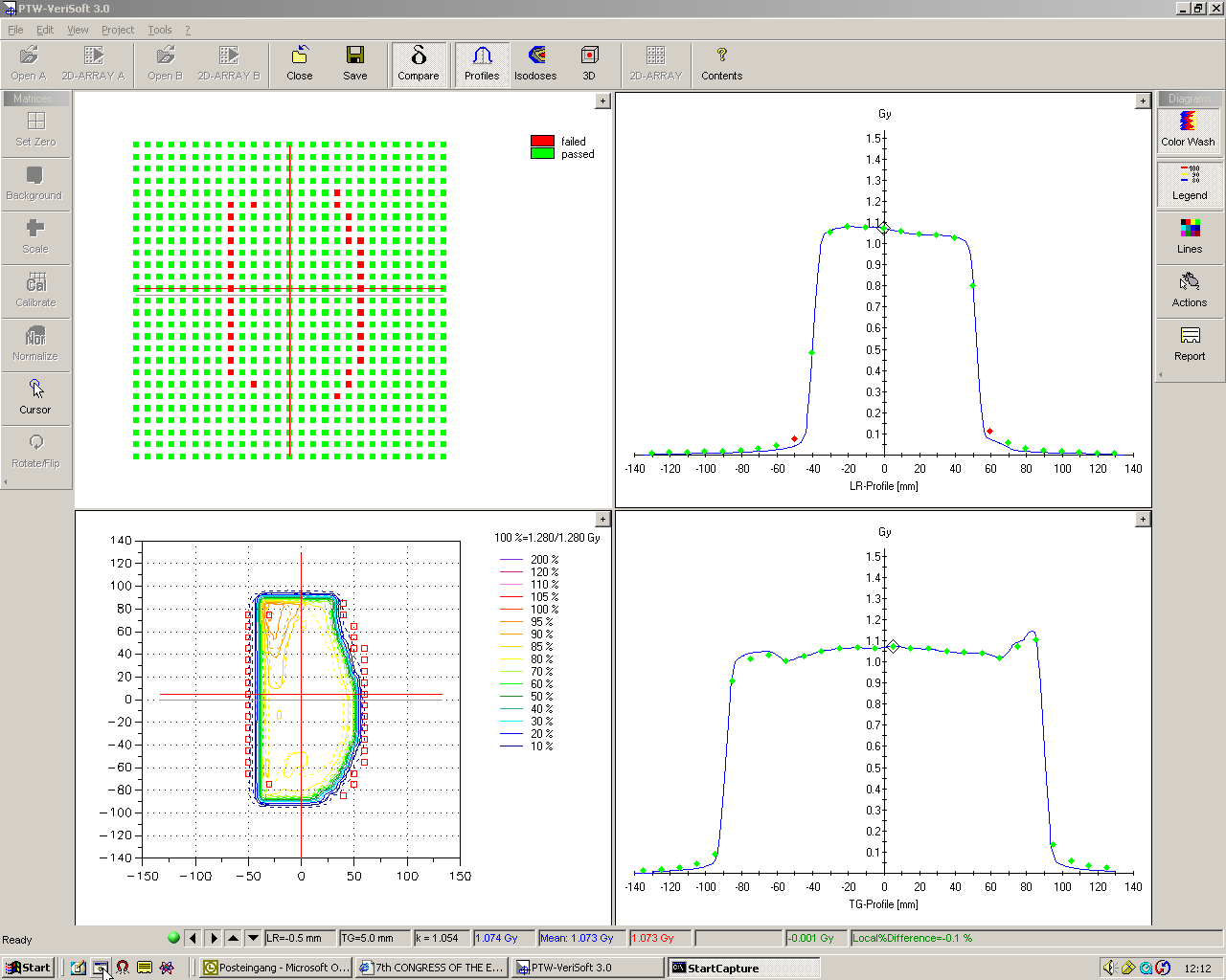
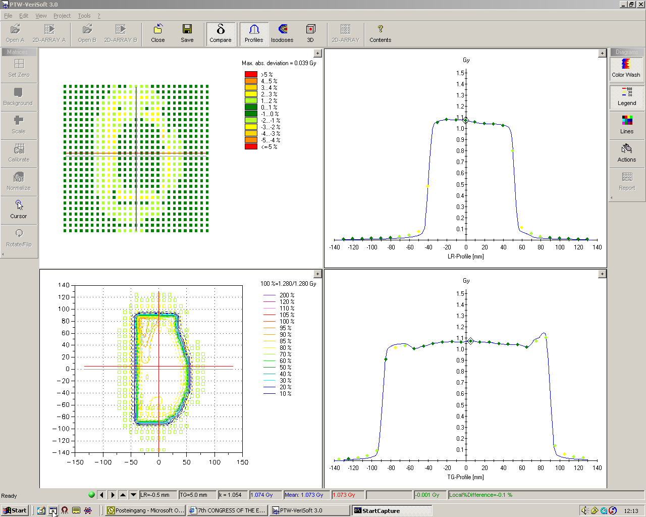
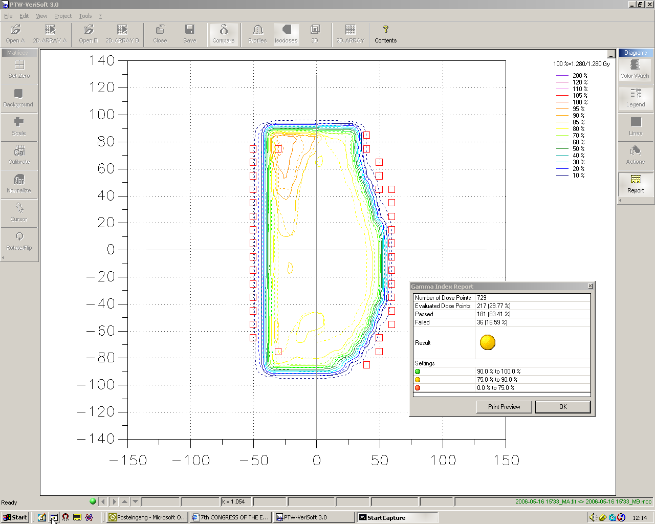
There are only two files for each field that need to be accessed on the linac: the dynamic MLC file and the planned dose file. The dynamic MLC file is loaded to the MLC controller, the dose file is opened with VeriSoft.