The Dark Side of the MU1
To our knowledge, beam ramp-up ("Einschwingen") of the TrueBeam has never been measured before. So we went to the basement and shook the dust off our fast measurement system which had not been used for a very long time. We were delighted to see that it was still in perfect working order2:
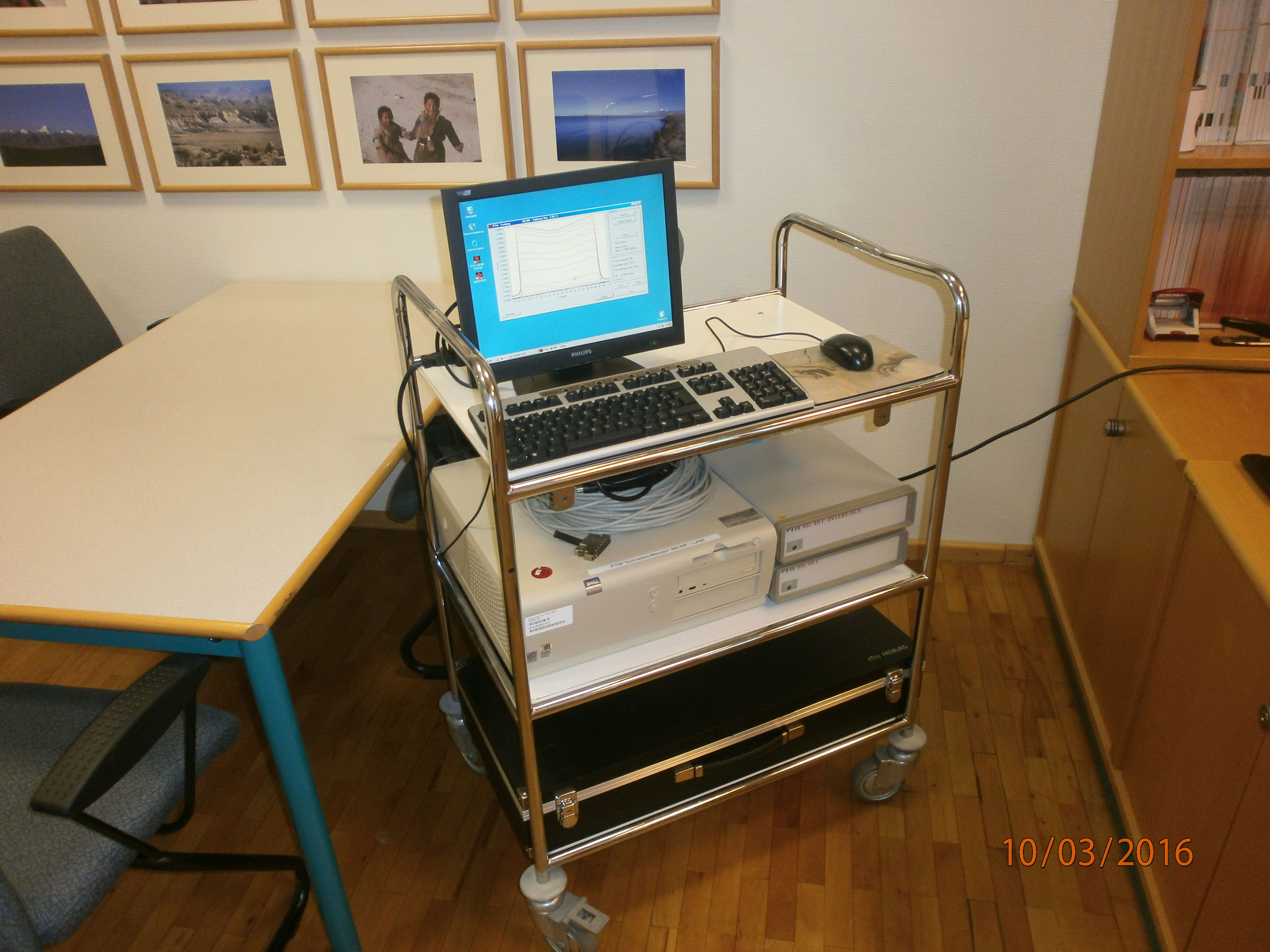
The fast measurement system ("Schnelles Messen") was offered by PTW in the nineties as an option to the LA48 linear array. Nearly nobody except us bought it, so the product was soon discontinued3. We think this is a shame. It is exciting for the physicist to use, and it gives confidence that the beam behaves as expected even at small time scales. It tickles us pink to be able to say that Schnelles Messen is still the fastest PTW measurement system. Compared to a STARCHECK with its 100 ms minimum measurement time, Schnelles Messen is faster by a factor of ten! When mounted on the dedicated AirScanner, measurements can be performed both with static and dynamic Gantry.
Schnelles Messen works for all energies over the full range of TrueBeam dose rates. We will give examples ranging from 6 MV @ 5 MU/min, over the 2.5 MV imaging energy at 60 MU/min, to the 10FFF energy at 2400 MU/min.
We described the principle seventeen years ago. Nothing has changed inside our "time capsule". Only the Clinacs have been replaced by TrueBeams in the meantime.
You may ask yourself: what is "The Dark Side of the MU?" Read on.
The Raw Data File Format of "Schnelles Messen"
Measurements are controlled via the ME48F software. We use version 1.03T, which is a test version.
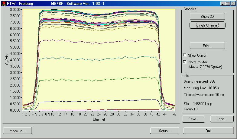
The last officially released version was 1.02.
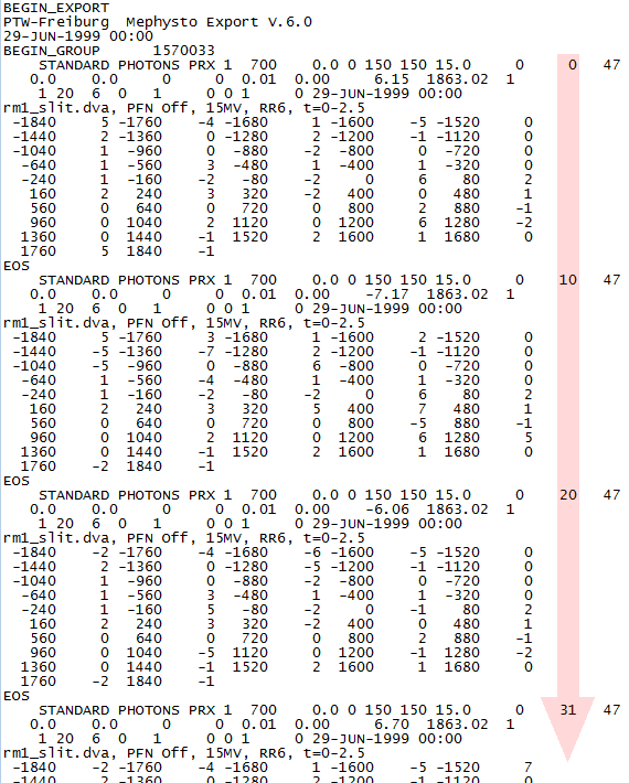
Raw measurement data is saved in PTW's standard text file format of the time, which has the extension "EXP". The beginning of a fast measurement looks like this. The red arrow covers the time stamp in milliseconds. The ME48F software saves time information to a field which is normally used for the off-axis distance.
When the EXP file is opened with a more recent version of Mephysto (MEPHYSTO mcc 3.2), it looks like this. The time stamp of each profile is in the last column. The value has to be multiplied by ten to give the correct time in milliseconds.
Data Manipulation
After each measurement, data was saved in EXP format on the measurement PC. At the end of the session, all files were copied via USB stick to a physics PC. There, the following sequence of data manipulations was performed for all files:
- The EXP file was opened with MEPHYSTO mcc 3.2 and wrong administrative data was corrected (e.g., FFF energies).
- All curves were smoothed once.
- The complete file was saved in MCC format.
- A second file, which typically contained the first 0.5 seconds of beam (50 profiles) was also saved.
- With a home made file conversion tool ("SchnellesMessen.exe" © M.Papauschek), the uncorrected data matrix was extracted from the MCC file, and saved in CSV format. The rows contain the profiles. Column 1 of the matrix contains the profile time stamp (named "t1" below), columns 2 to 48 contain the profile data.
- With MATLAB, the CSV file was imported, the readout time correction (see below) performed, and plots generated.
- In MATLAB, the corrected matrix was again saved as CSV file, in the same format as in step 5.
- With SchnellesMessen.exe, the corrected data matrix was merged into the MCC file of step 3.
- The MCC file now contains corrected data and can be opened with MEPHYSTO mcc 3.2 for further analysis (e.g., symmetry, see below).
Correction for Finite Readout Time
The 47 chambers of the LA48 are read out sequentially. Due to the finite readout time of 2 ms per profile, the time stamp is not valid for the whole profile. For simplicity, we assume that the time stamp as it appears in the data file is the time stamp of chamber 1 ("t1").
We do the necessary correction in MATLAB. For each chamber, we interpolate the measured values linearly between two successive profiles, which are 10 ms apart. The measurement values of chamber 1 are the only ones which need no correction (see assumption above). Chamber 2 has a true measurement time stamp of t2 = t1 + 43.5 µs, and chamber 47 has a time stamp of t47 = t1 + 46 * 43.5 µs = t1 + 2 ms. By linear interpolation, the measured values of all chambers at the same time t1 are computed.
The correction is large when the change in dose rate is large (beam rise and beam fall). For the same dose rate gradient, the correction increases linearly from left to right. The correction is zero when dose rate is constant (at a ridge or plateau).
The next image shows the front face of a 10 MV beam rise, uncorrected on the left, corrected on the right. The two red helper lines mark the first two profiles above noise level, 10 and 20 ms after the beam has started to rise:
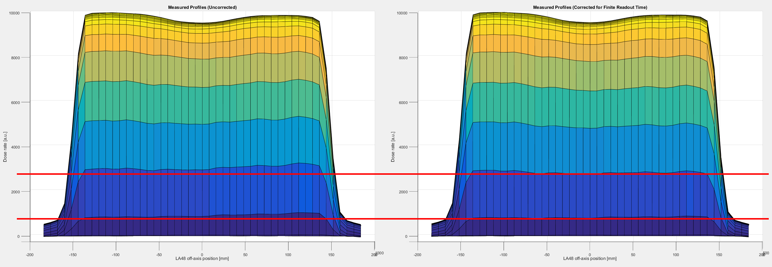
If misinterpreted, the inclined uncorrected profiles could be attributed to the TrueBeam, but this is wrong. It can easily be checked whether the effect comes from the measurement system or the linac, by turning around the LA48 and repeating the measurement.
In the example of a 10 MV beam ramp-up (right plot), the beam first rises and reaches the nominal dose rate (100% = 600 MU/min) 60 ms later. It overshoots to 110%, stays on this plateau for a while, and then settles at the nominal dose rate 198 ms after beam-on:
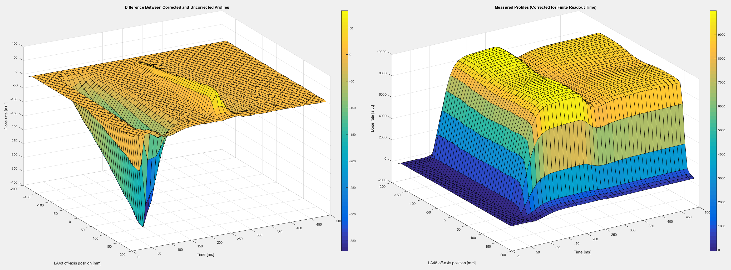
One should know that when the measurement is repeated, it may look slightly different. It depends on the action of the servos. Therefore, the right plot must not be understood as a "signature" of the 10 MV beam.
The left plot shows the magnitude of the readout time correction. During beam rise, the correction is negative and increases from left (no correction for chamber 1 at -184 mm) to right (maximum correction for chamber 47 at +184 mm). At the small dose rate drop, the sign of the correction is reversed.
As mentioned in our blog entry from 1999, PTW has tested Schnelles Messen on a Siemens machine, which defined the developer's frame of reference regarding beam rise times. They found no distortion coming from the measurement system. Therefore, the PTW software does not correct for finite readout time.We won't mention the readout time correction any further. All measurements presented here are corrected.
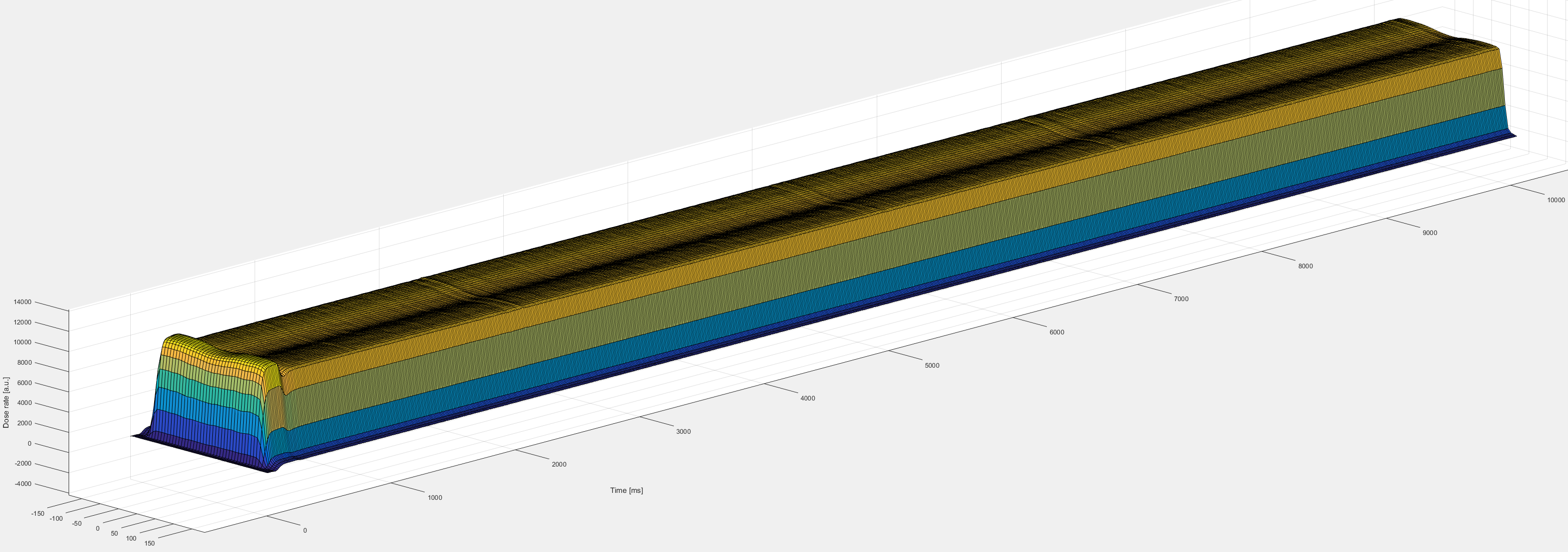
Usually, all the interesting things happen within the first second after beam-on, when the servos start to work. We will focus on that. Longer measurements are usually boring, and hard to plot:
A Word on Absolute Units
The LA48 is calibrated both electrically and radiologically (60Co calibration). The measurement software uses two calibration files and also displays dose rate in units of Gy/s on the screen. When the measurement is saved as an EXP file, the absolute dose information gets lost.
However, this is not a problem. We are not interested in absolute units. It would not give any extra information. Sometimes, we measure without buildup, sometimes with buildup, with different field sizes, and all these settings affect absolute dose. If this increases comfort, one can always think that the stabilized dose rate corresponds to the "nominal dose rate" of 60, 600, 2400 or whatever MU/min.
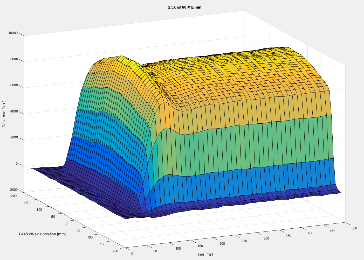
The 2.5X LowMV Imaging Energy
Regarding its Einschwingen, the LowMV imaging energy is not different from the other energies. Only one dose rate setting (60 MU/min) is possile. This value is reached after 55 ms. The profiles look a little noisy:
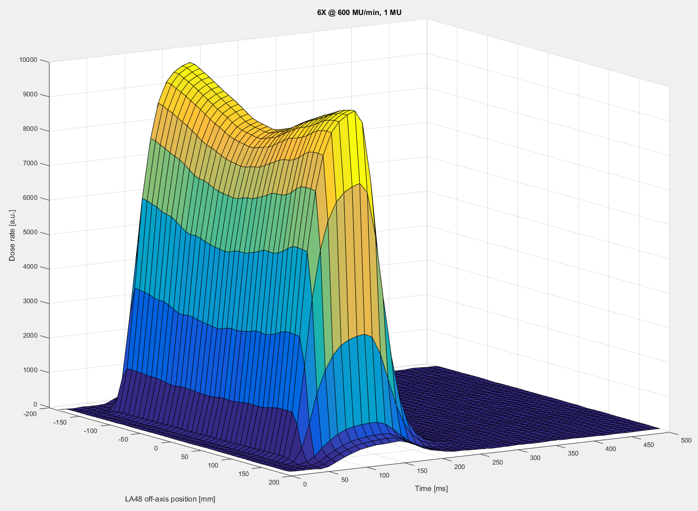
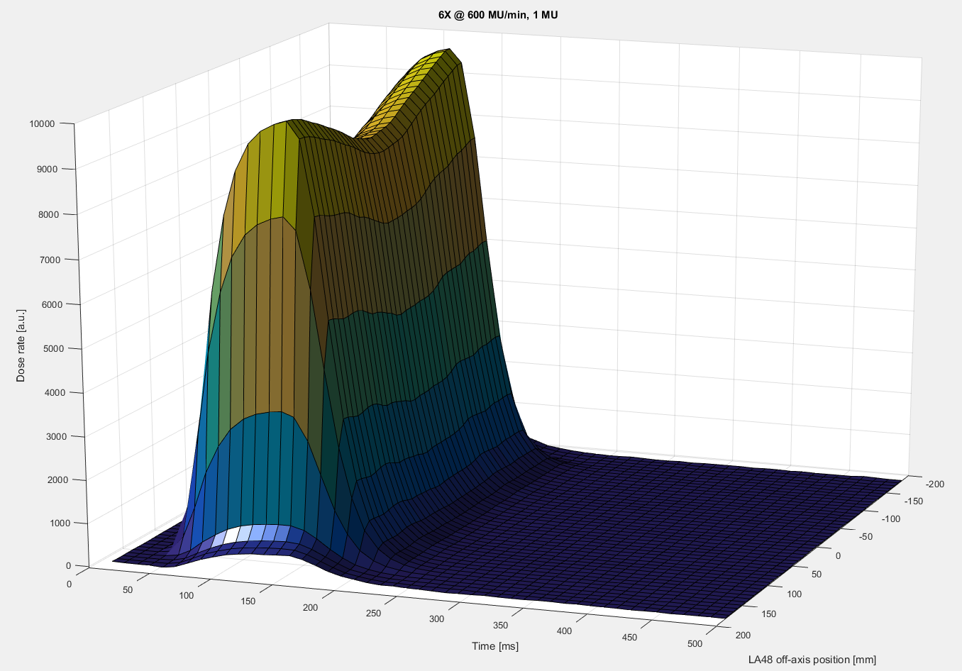
The 6 MV Flattened Energy
The Einschwingen of the flattened 6 MV energy at dose rate 600 MU/min, at least for this specific run, is just perfect. There isn't any overshoot. At other energies, a similar perfection is normally only seen when dse servo is switched OFF. This is why we have written it explicitely in the title of the plot. Here the dose servo was ON, although it looks like it was OFF:
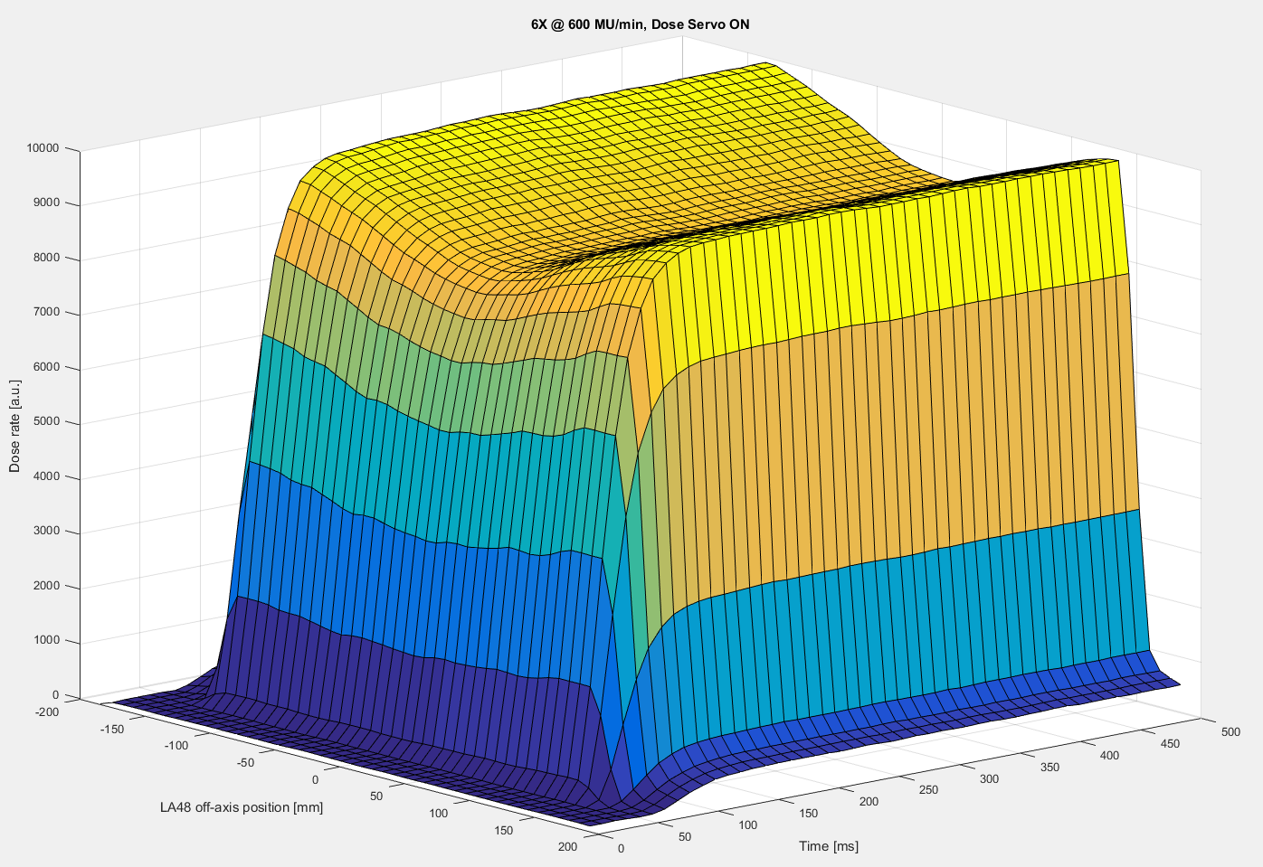
There is no error possible. For 6 MV and dose rate 600, dose servo cannot be switched off.
Extremely Low TrueBeam Dose Rates
Besides the standard set of dose rates of flattened photon beams (100 - 600 MU/min), TrueBeam can deliver dose at much lower rates. These modes produce no stable beam, but rather single short bursts of radiation. The next plot shows the first 0.5 seconds of beam, which consists of three single pulses. Nominal dose rate is 10 MU/min:
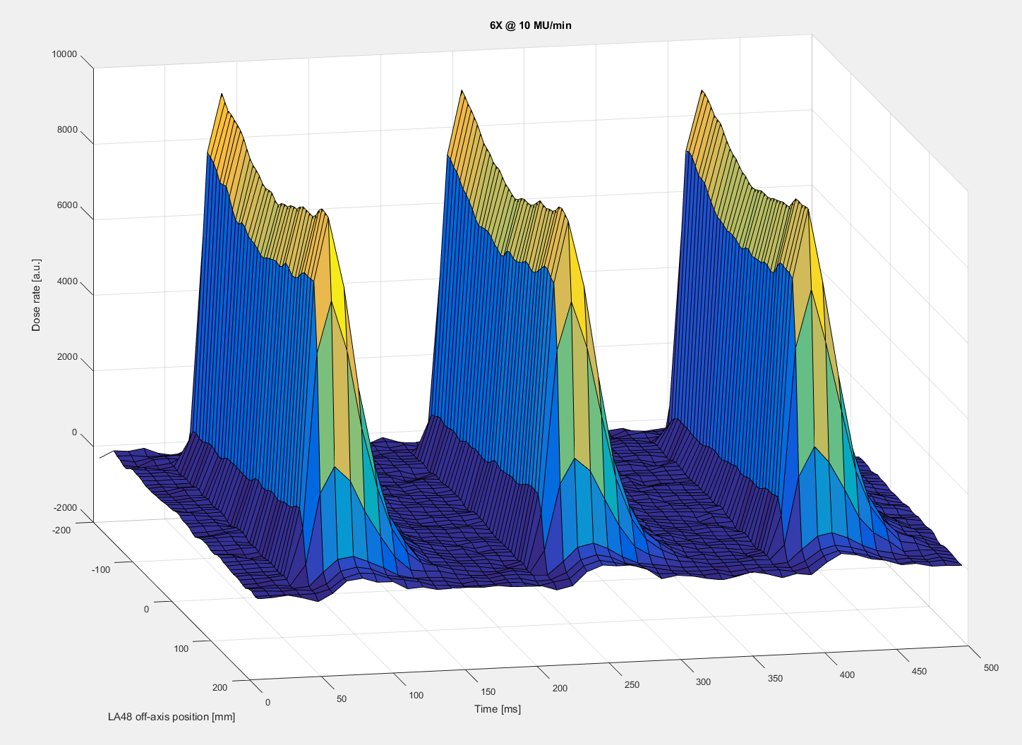
The shape of the surface depends a little on the measurement settings. Here is another run with the same linac settings and a slightly different trigger level for auto start:
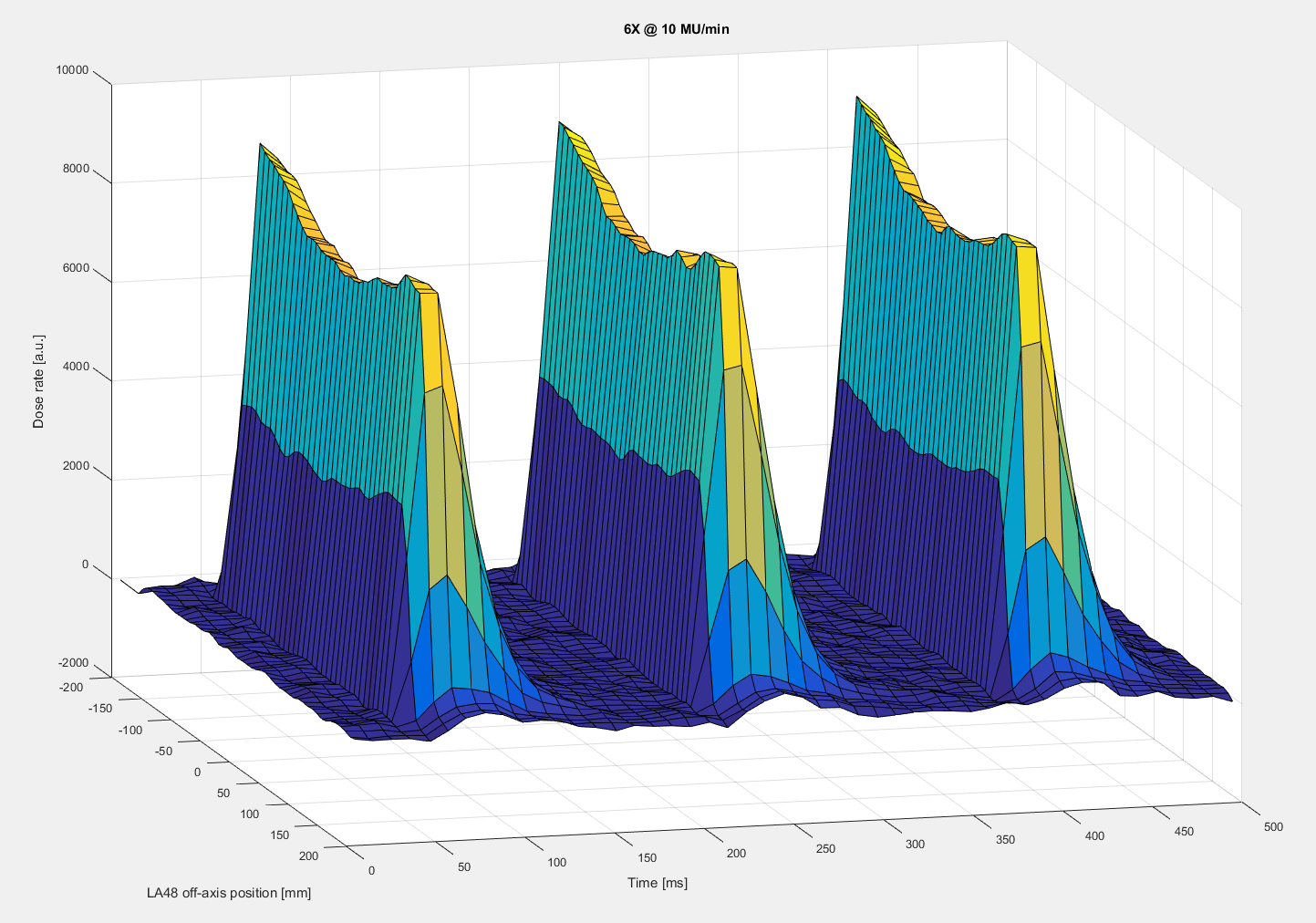
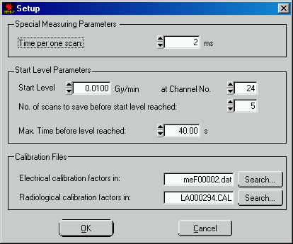
When the dose rate of the start level is reached, the measurement clock starts ticking. However, a certain number of profiles before that are also saved (in the screenshot, this number is five).
It is possible to go even lower. The next plot shows the lowest clinical dose rate that can be set on the TrueBeam: 5 MU/min (We have no idea what the clinical application might be):
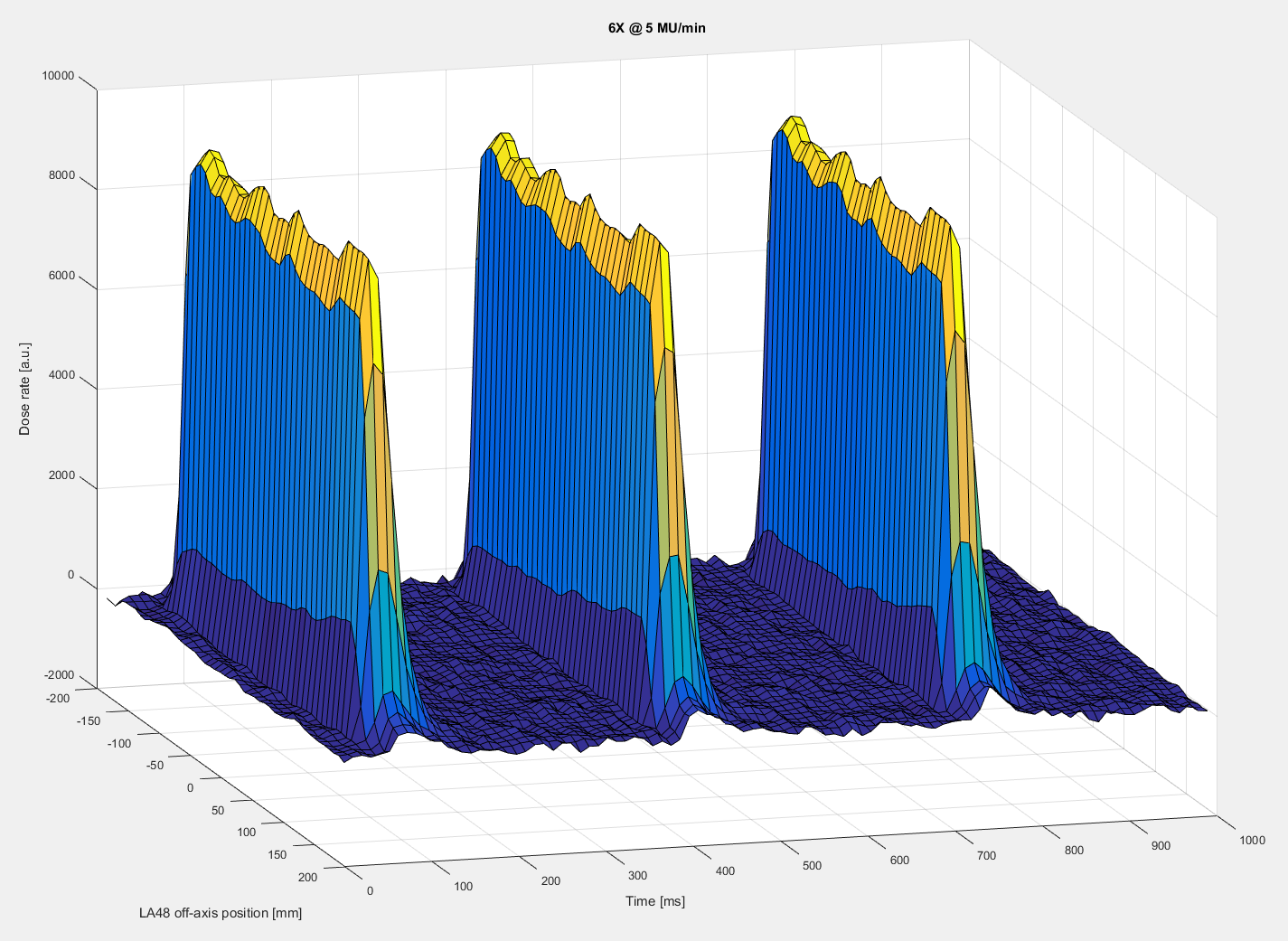
Still three pulses, but the time axis now goes to 1 s, not 0.5 s. And the noise level is rather high. Dose rate at the ridge of the pulse peaks was about 0.25 Gy/min.
The Effect of the Dose Servo
During clinical treatments, the dose servo is always ON. The servo control makes sure that dose rate is always at nominal. When the dose servo is switched OFF in Service Mode, the dose rate rises by about 10 to 15%. If the nominal rate is 600, it will go up to about 700 MU/min.
The servo's control action can be seen with Schnelles Messen. Servoed dose rate sometimes produces ripples on the surface, while unservoed dose rate surfaces are flat.
Some Examples
6FFF, dose rate 1400 MU/min, dose servo ON, the first 0.5 s:

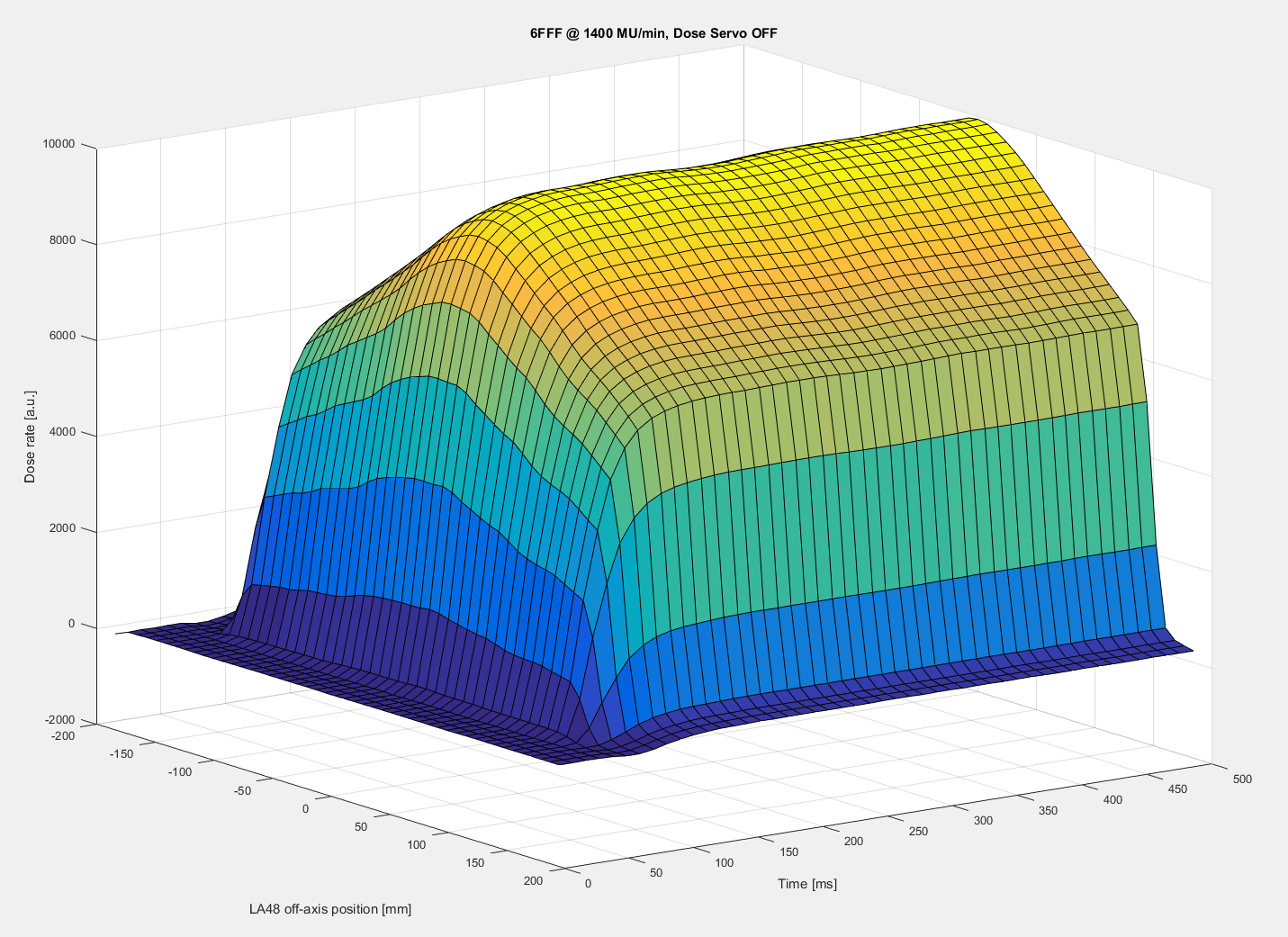
6FFF, dose rate 1400 MU/min, dose servo OFF, the first 0.5 s:
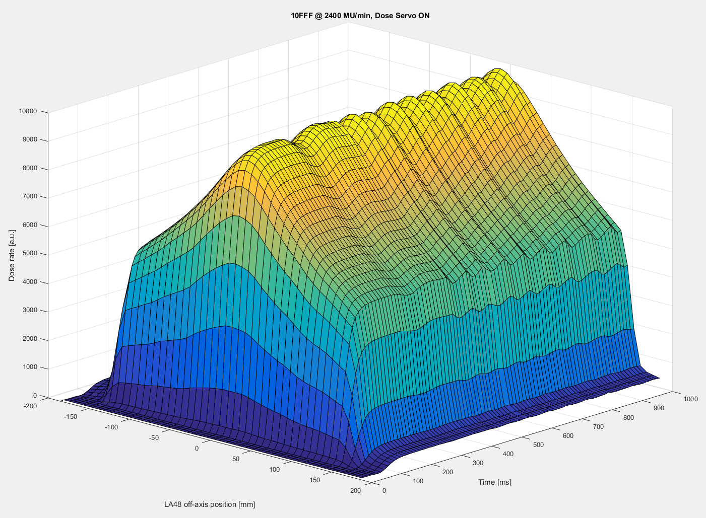
10FFF, dose rate 2400 MU/min, dose servo ON, the first second:
10FFF, dose rate 2400 MU/min, dose servo OFF, the first second:

Symmetry Analysis
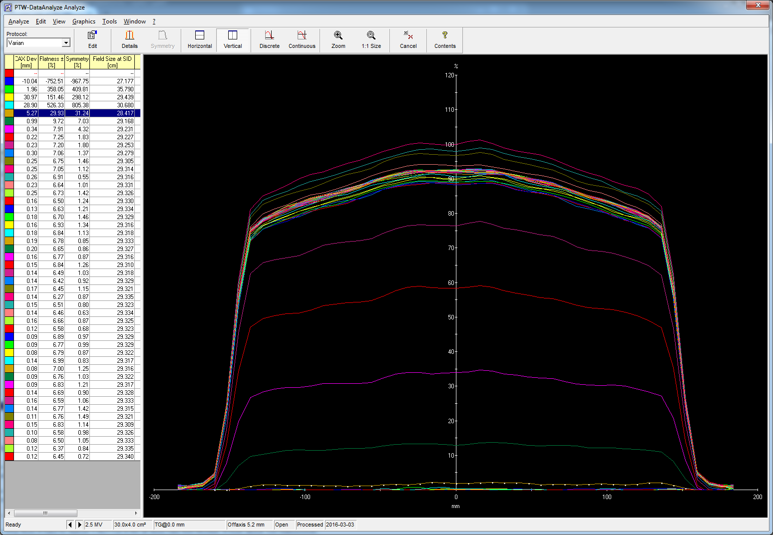
It is interesting to know the symmetry of the ramping beam. We analyse the MCC file described in steps 8 and 9 of the Data Manipulation section above. We use the Varian protocol, where symmetry is defined as the maximum variation (D(x)-D(-x))max.
We directly jump to the most demanding beam, the 2.5X imaging energy with 60 MU/min, and check symmetry.
Strictly speaking, the 2.5X is a flattening filter free (FFF) energy. However, declaring the energy in MEPHYSTO mcc 3.2 as "FFF" will not work, because in order to get the FFF specific analysis results like unflatness, slope, peak position etc., certain renormalization values are needed. They are not implemented for 2.5X.
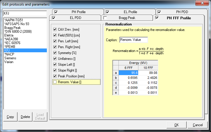
In order to get any result, we therefore have to pretend that the 2.5X is a flattened energy. Then we can use the standard protocols.
The last profile before the beam rises above noise level is at 52 ms (see "Offaxis" value in the status bar at the bottom of the screen shot, which has to be multiplied by ten):
Varian's symmetry specification for 2.5X is 3% for a beam which has stabilized. Three profiles later, at 83 ms (or 30 ms after the beam has started to rise) the symmetry of the beam is already within specs:
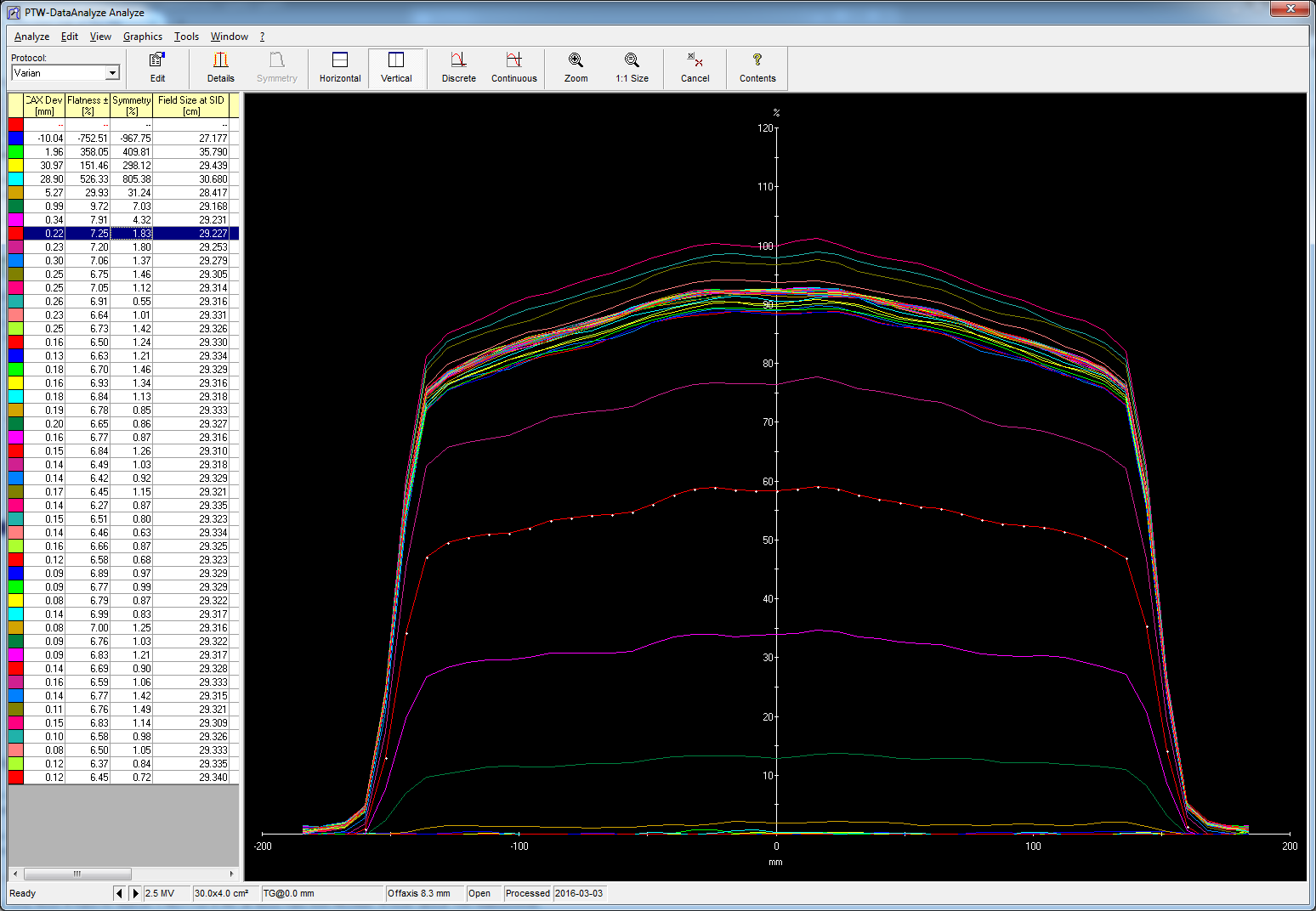
If one takes into account the low spatial resolution of the scans (8 mm distance between the LA48's chambers) and the noisy data, this is a very good result. There is no indication that the profiles between 52 and 83 ms are NOT symmetric. They are just too noisy.
The Einschwingen of the 6FFF beam at 1400 MU/min is shown in the following animation (compared to real-time, it is slowed down by a factor of ten):
Time in the animation runs from 0 to 500 ms. The beam starts to rise at 41 ms. At 104 ms (63 ms later) symmetry is neary perfect at 1.04%. Varian's specs is 2% for the stable beam.
Photon beams of the TrueBeam during Einschwingen seem to be symmetric right from the onset of measureable beam output. With an improved sensitivity of Schnelles Messen, noise in the data could be reduced.
Measurements of One MU
How long does it take to deliver 1 MU? For 6 MV at dose rate 600 MU/min, it took about 190 milliseconds.
How do we know? Well, WE have all the information available in different formats, and in different software. But you can easily find out by yourself, simply by counting the profiles on the 3D surface plots. On the front side (up to the ridge), there are 10 profiles above noise level (we also count the one which is slightly above zero):
All we then have to do is to turn the MU around, and count the profiles on the back side.
There it is! The Dark Side of the MU! And it is REALLY dark:
(We gratefully accept the Nobel prize for this discovery ...)
Notes
1To get the pun, MU should be pronounced as "Moo", not "Em-You".
2The computer clock was off by only five minutes after 16 years.
3In the age of 2D-Arrays, the same seems to happen to linear arrays right now.