Preparation in Eclipse
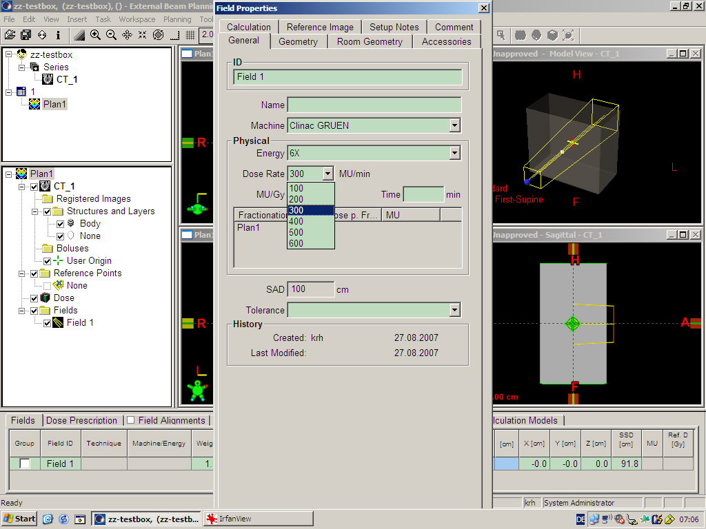
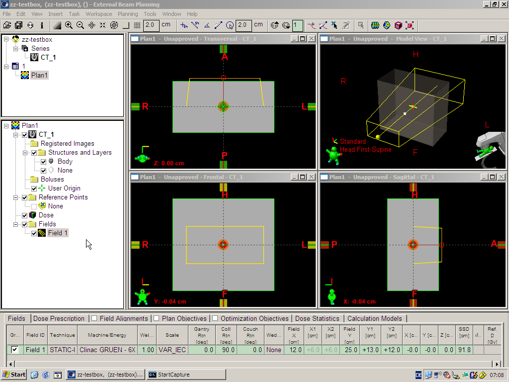
Open a test patient in Field Setup workspace of External Beam Planning, create a new plan with one field and the energy that shall be configured (on this page it is assumed that the energy will be 6MV).
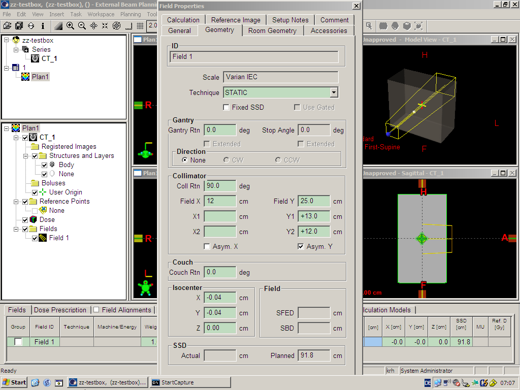
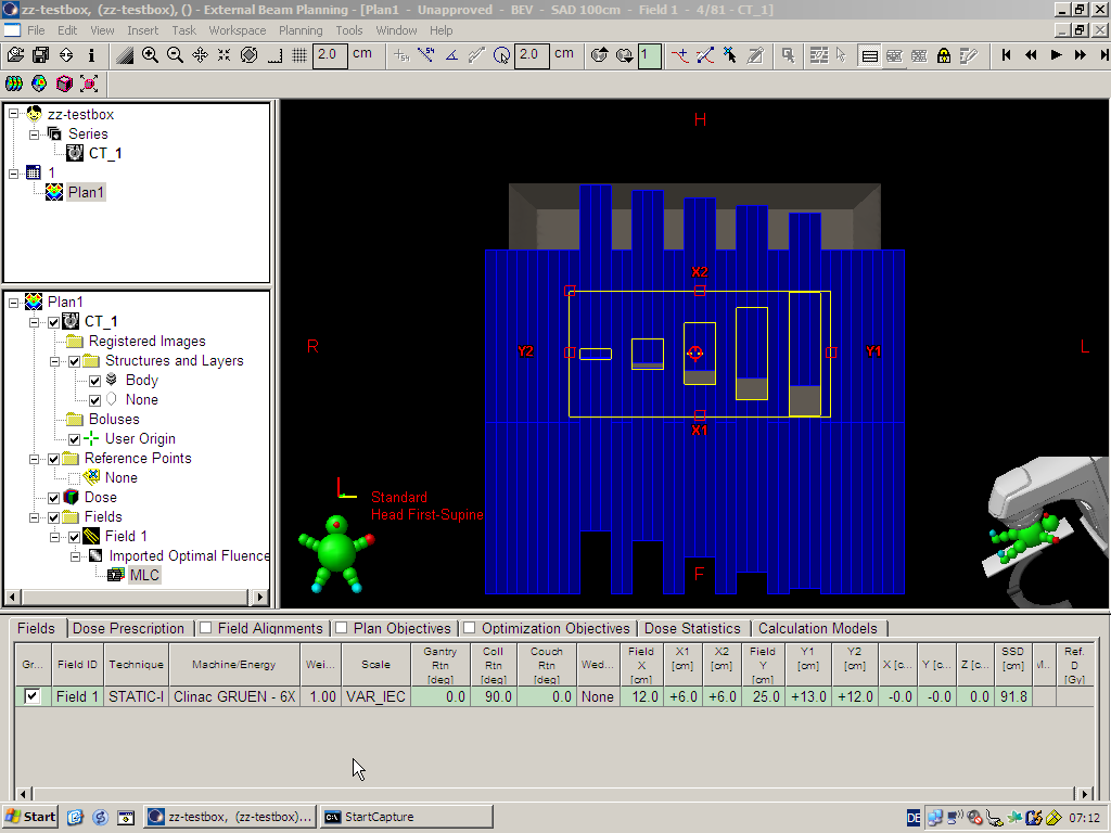
The field parameters are:
Gantry Rtn |
0° |
|---|---|
Coll Rtn |
90° |
X |
12 cm |
Y1 |
13 cm |
Y2 |
12 cm |
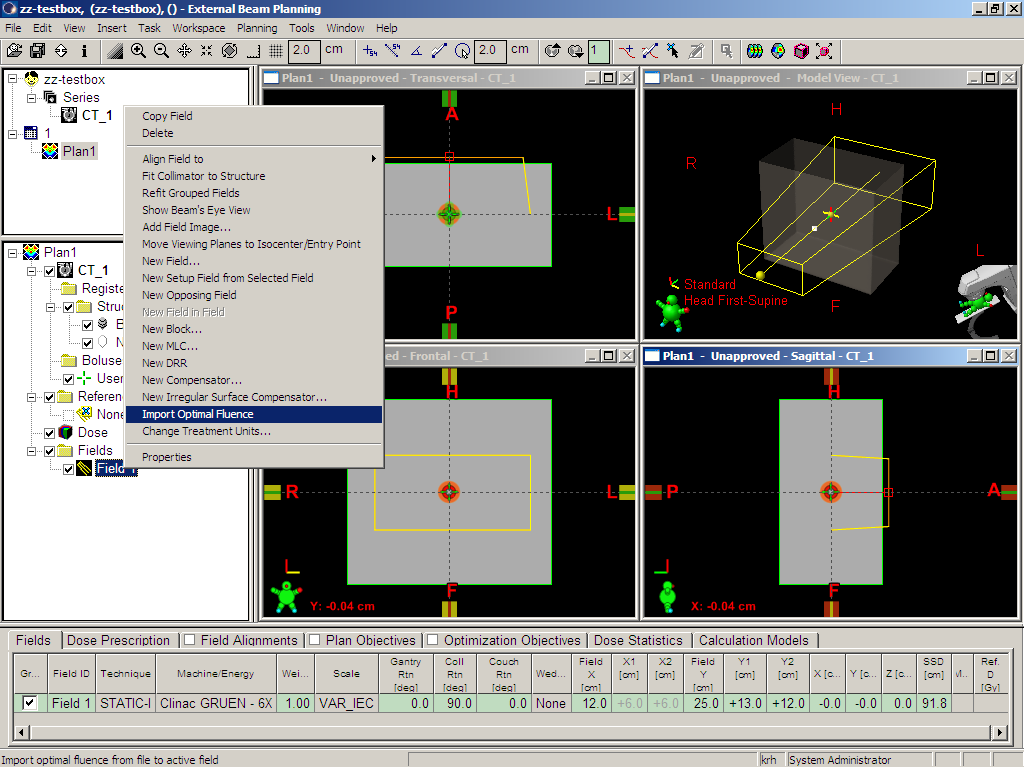
Right-click on the Field and select "Import Optimal Fluence". The corresponding fluence file can be downloaded here (right-click to save the ZIP-file to disk. The file "PDIP-configuration.optimal_fluence" is a text file and can be opened with a text editor).
Dose Prescription shall be 1.0 Gy per Fraction. The total number of fractions shall be two, because we need to aquire two images at different detector distances: 105 cm and 140 cm.
Plan normalization method shall be "No normalization".
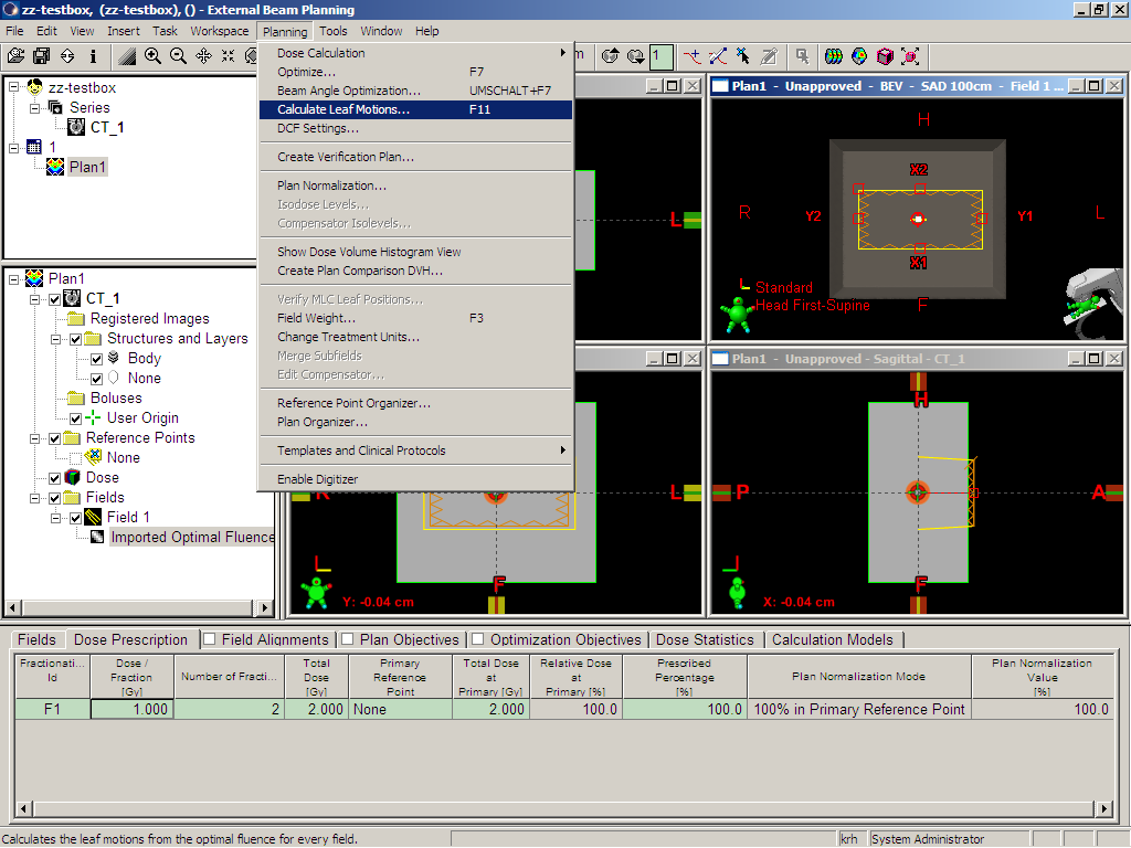
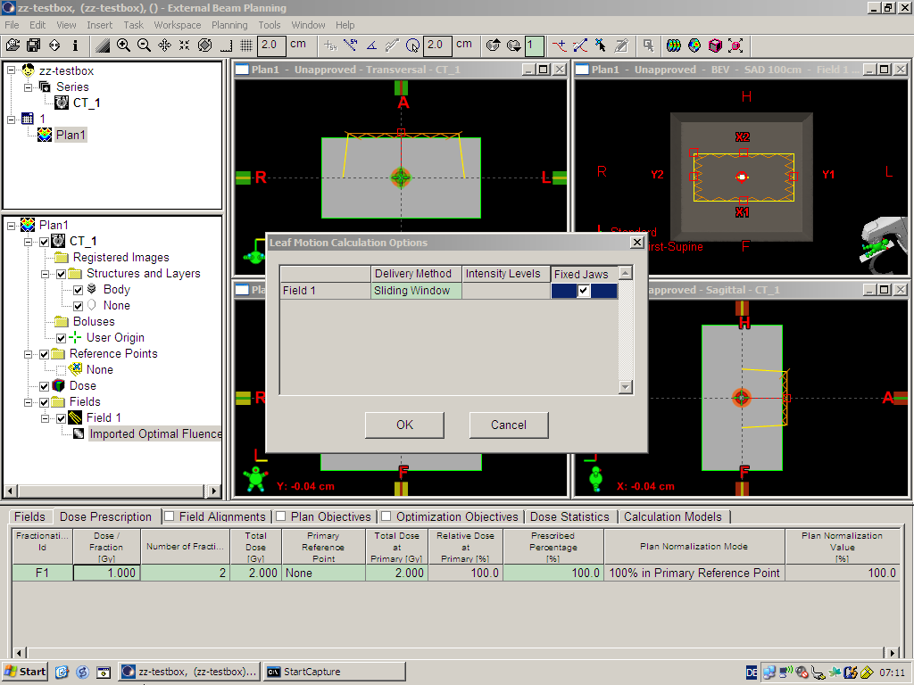
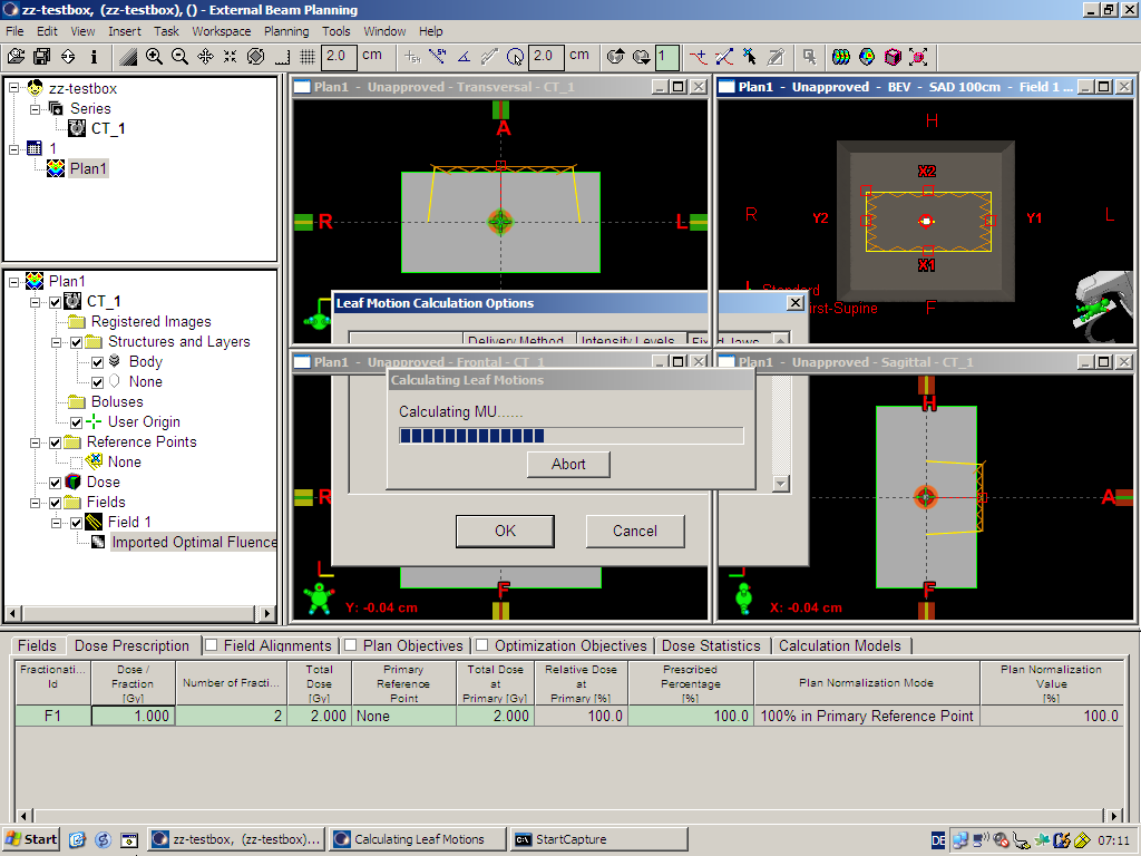
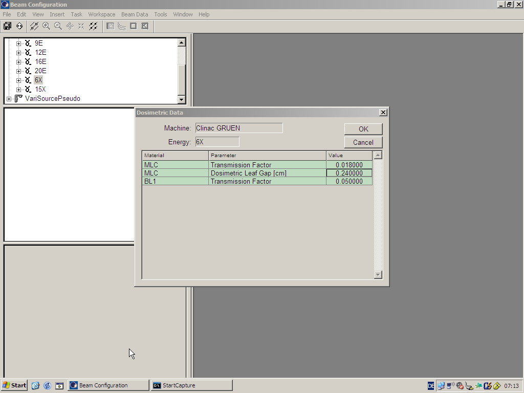
Leaf Motions are calculated next (F11), with "Fixed Jaws" checked. At this stage, the static MLC calibration and Dosimetric Leaf Separation have to be configured properly in Beam Configuration! Otherwise the calculated Actual Fluence and the resulting image will not be correct.
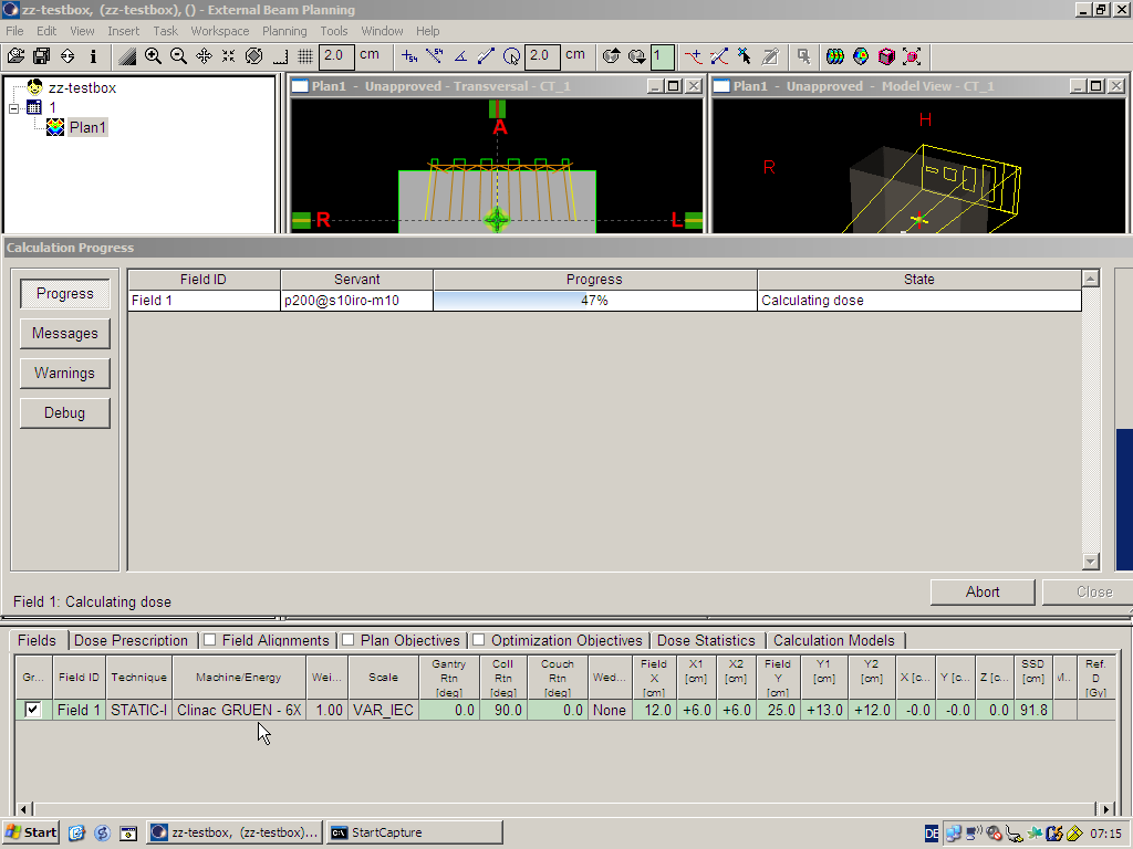
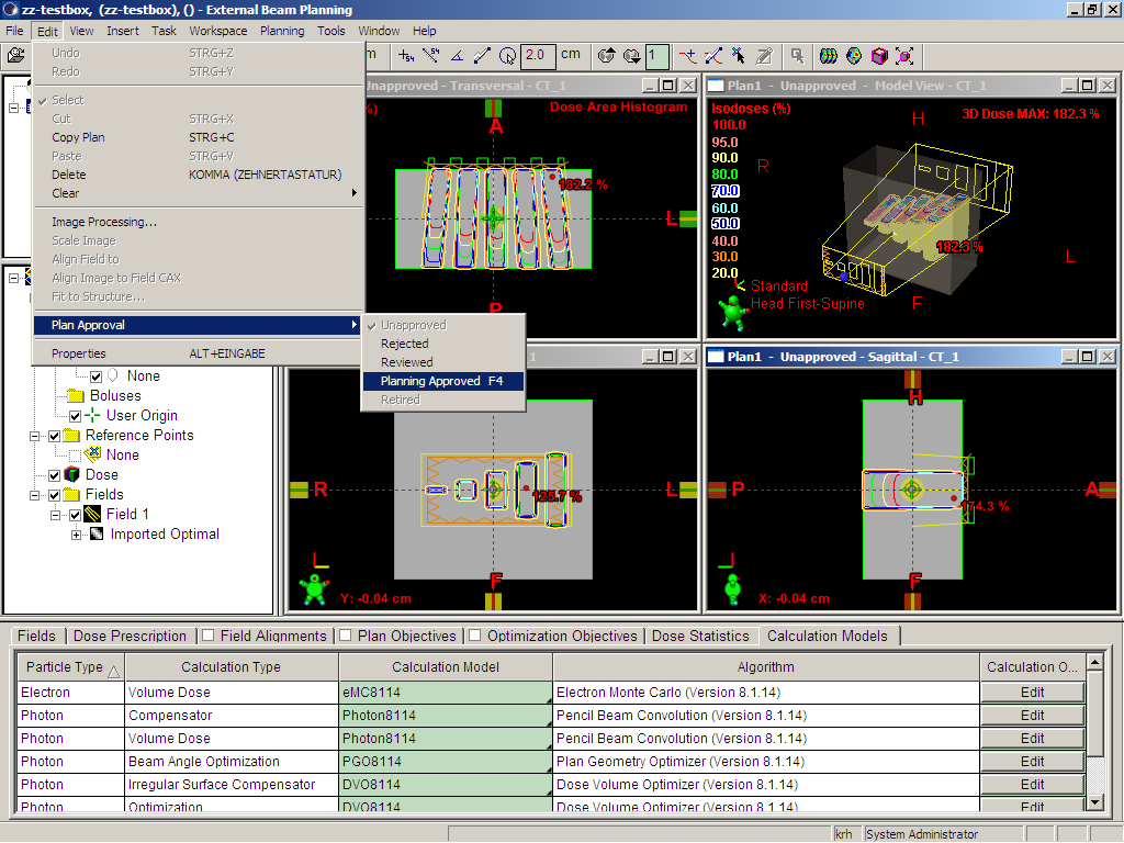
Calculate dose, save the plan, Planning Approve it (F4), and switch to RT Chart to finalize the plan for treatment.
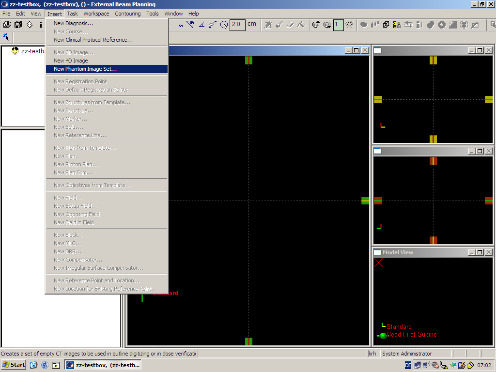
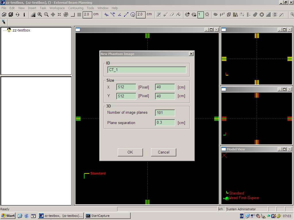
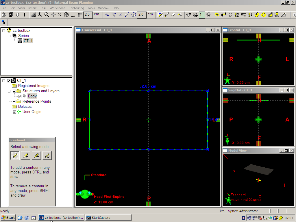
generate phantom image
select number of slices
draw rectangle
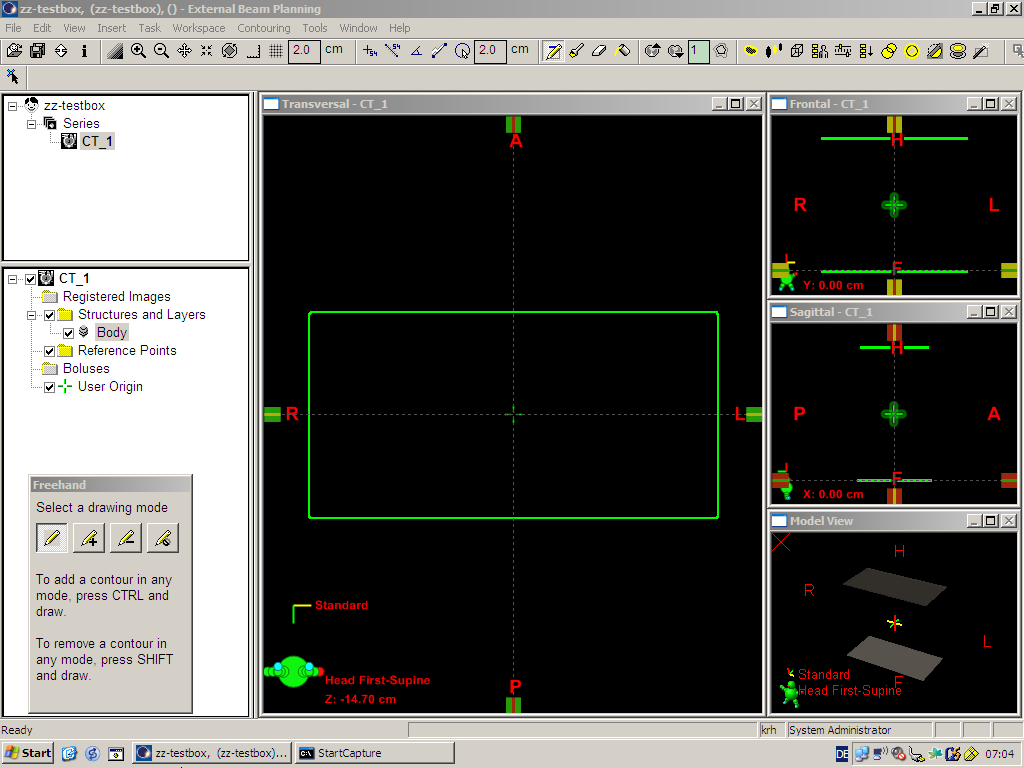
copy and paste rectangle
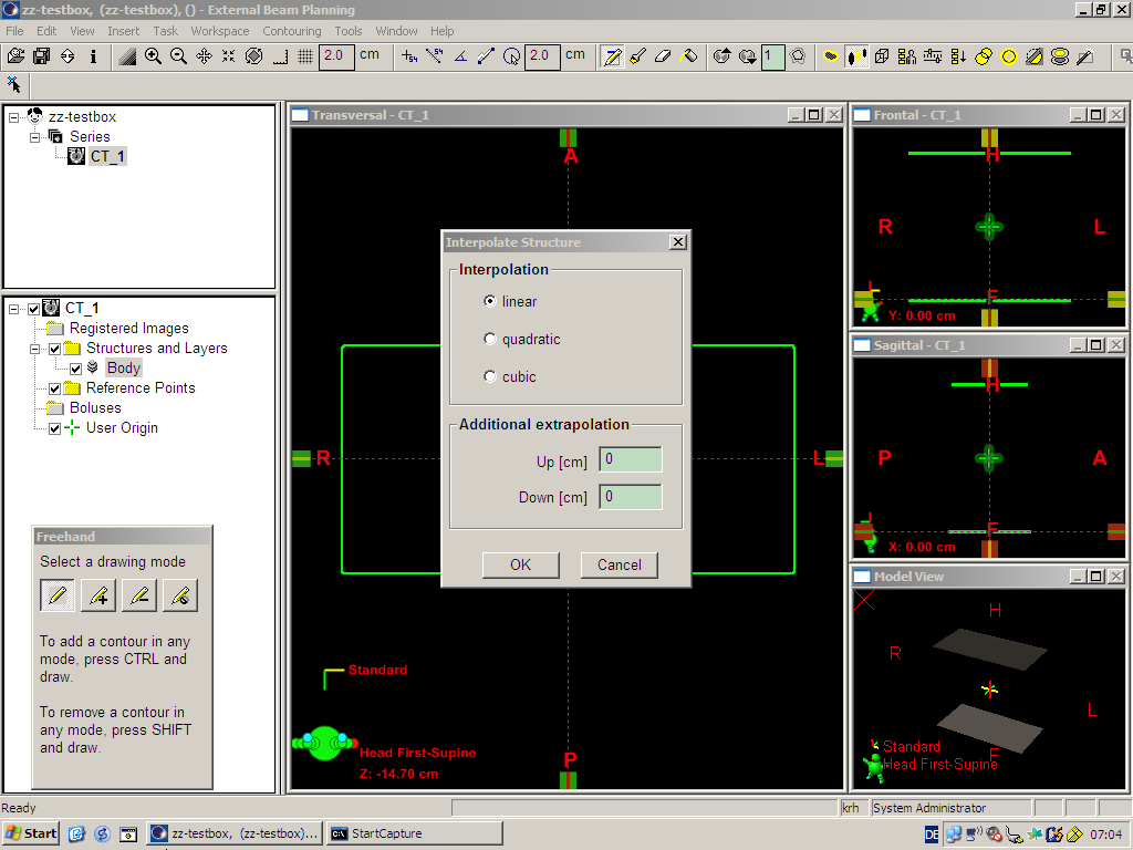
interpolate missing slices
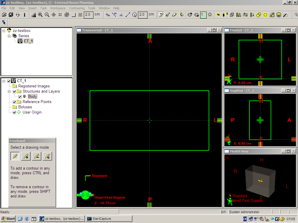
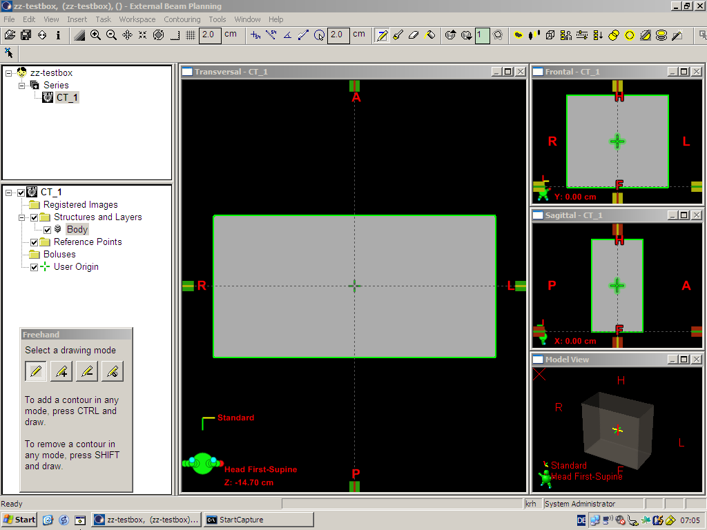
structure complete
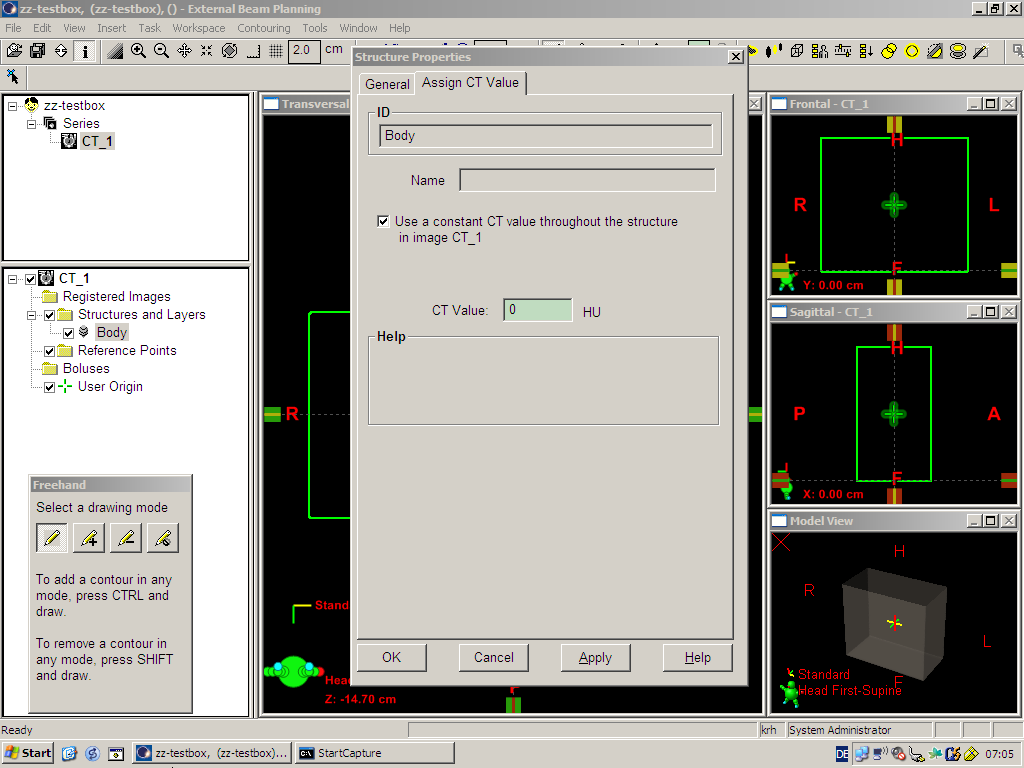
fill with 0 HU
body finished
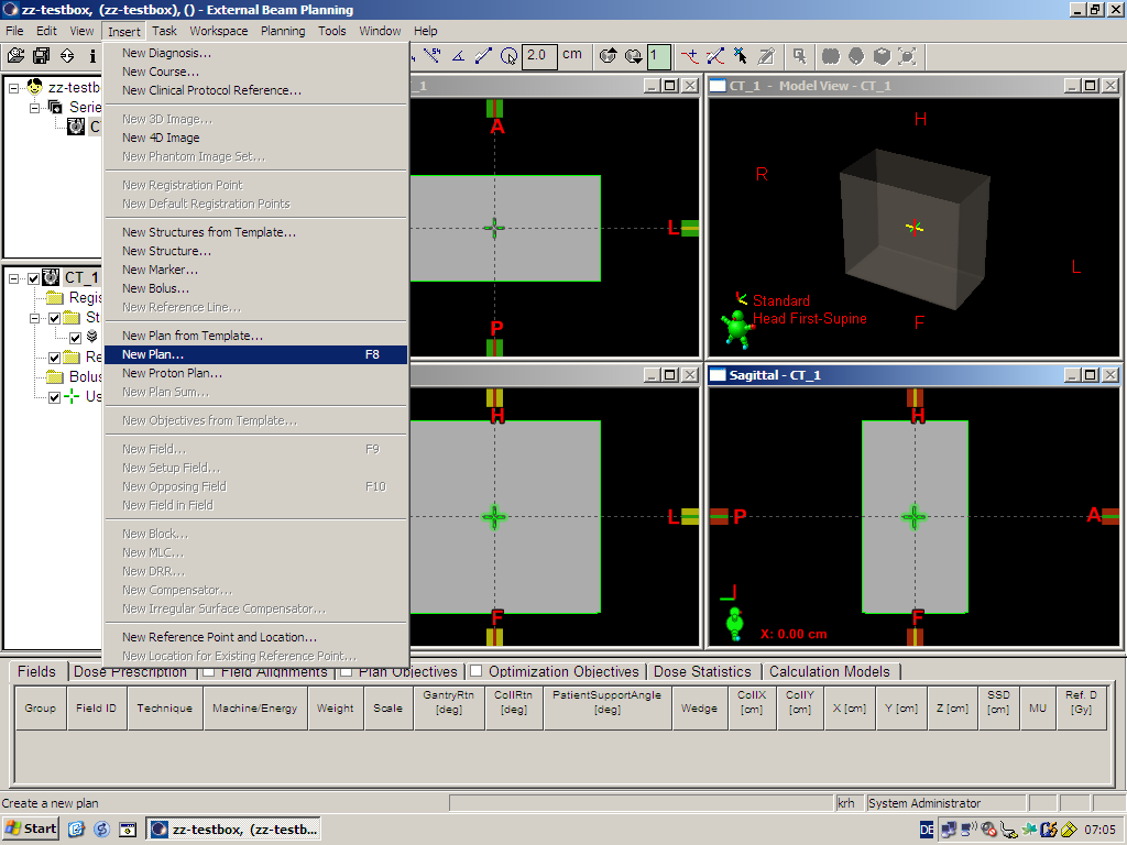
generate new plan
select energy and dose rate
enter field size
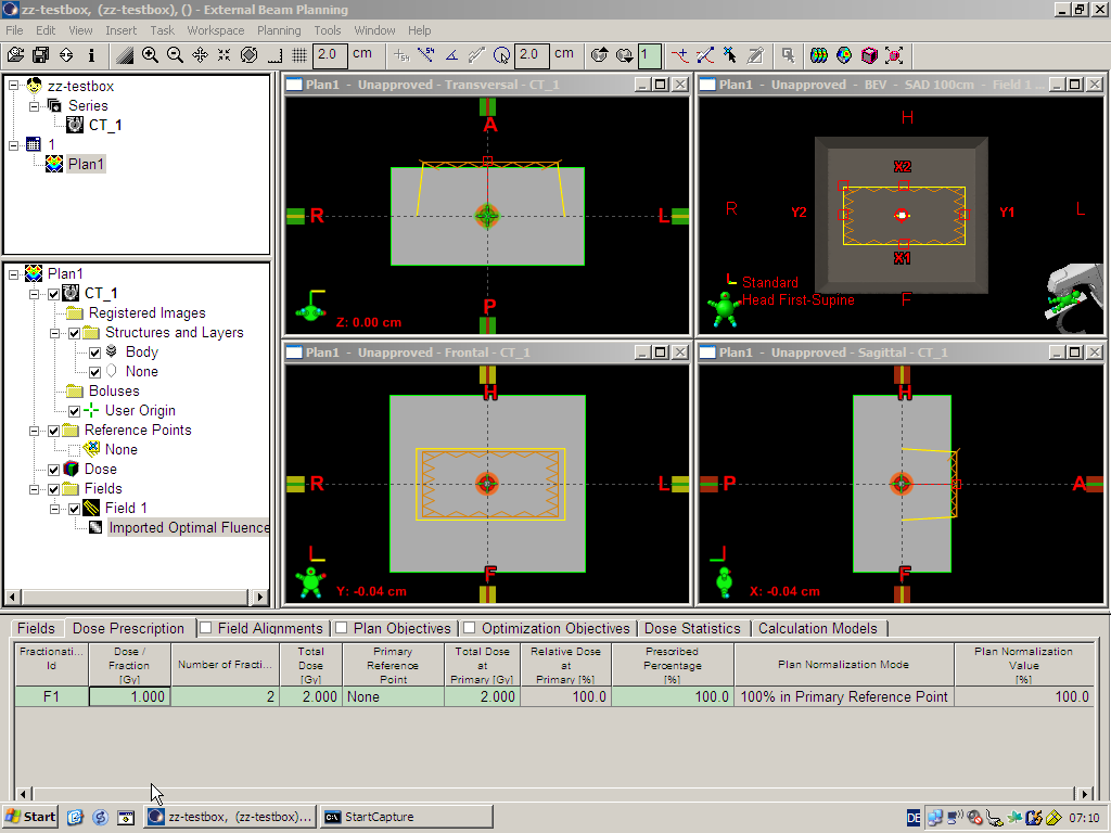
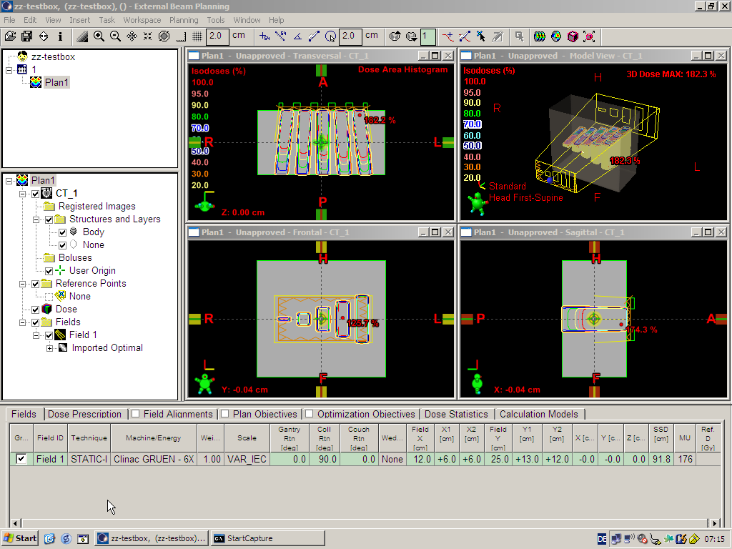
field overview
import optimal fluence
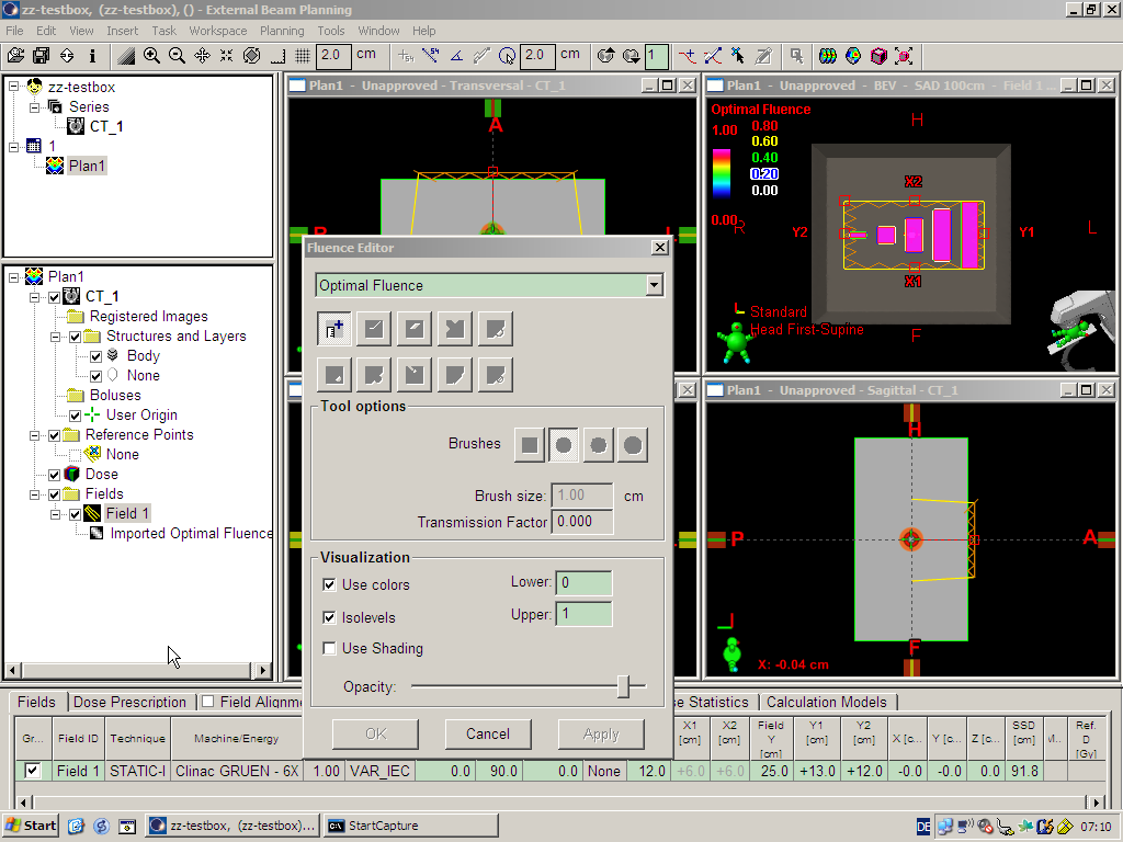
view optimal fluence
enter dose prescription
select calculate leaf motions
check fixed jaws
calculate leaf motions
visualize leaf motions
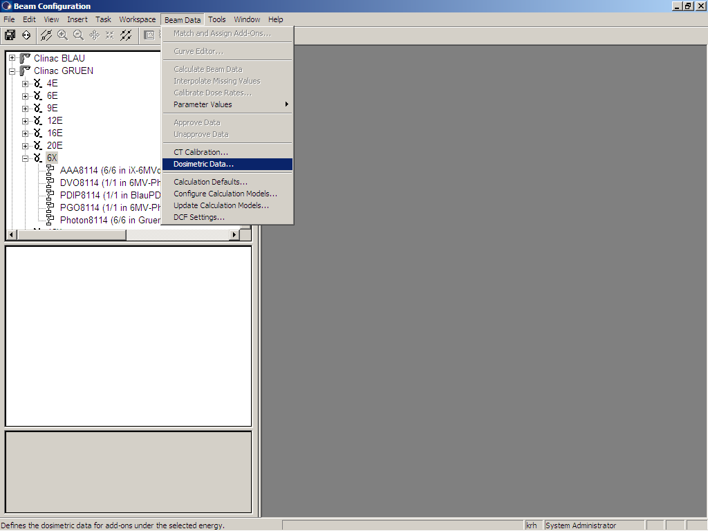
check dosimetric data
in Beam Configuration
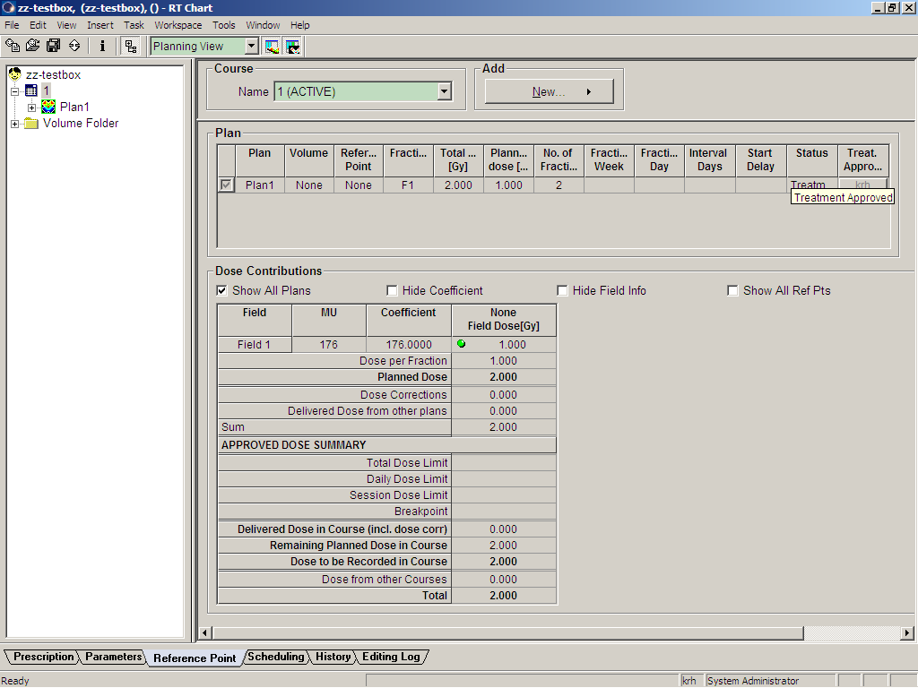
calculate dose
get 176 MU
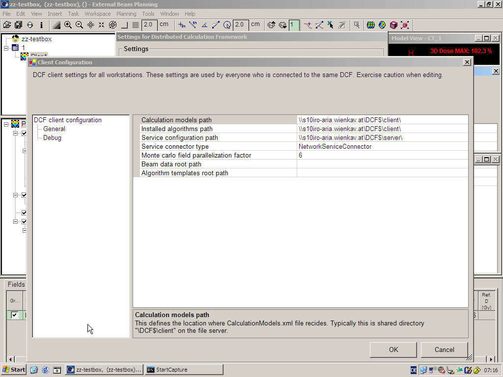
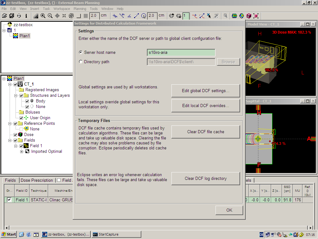
inspect Global DCF settings
DCF settings overview
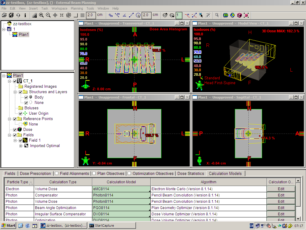
model is Photon8114
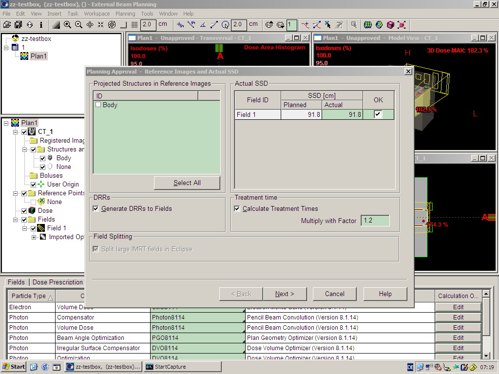
planning approval
enter time factor
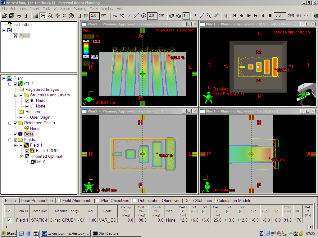
visualize dose
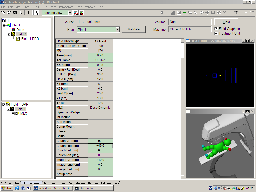
RT-Chart
In RT-Chart > Parameters tab, enter a Tolerance Table that will cause you no trouble during delivery. Enter couch parameters like Couch Lng = 40 cm, Lat = Vrt = 0 cm. The couch has to be out of the way during delivery.
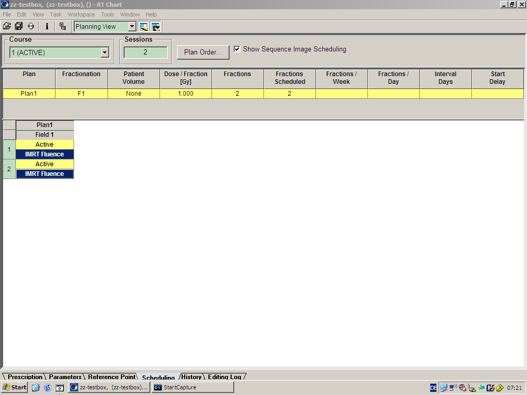
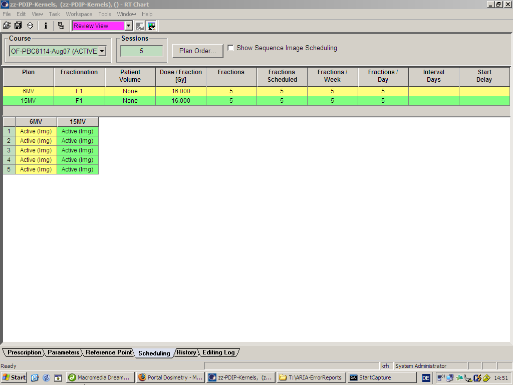
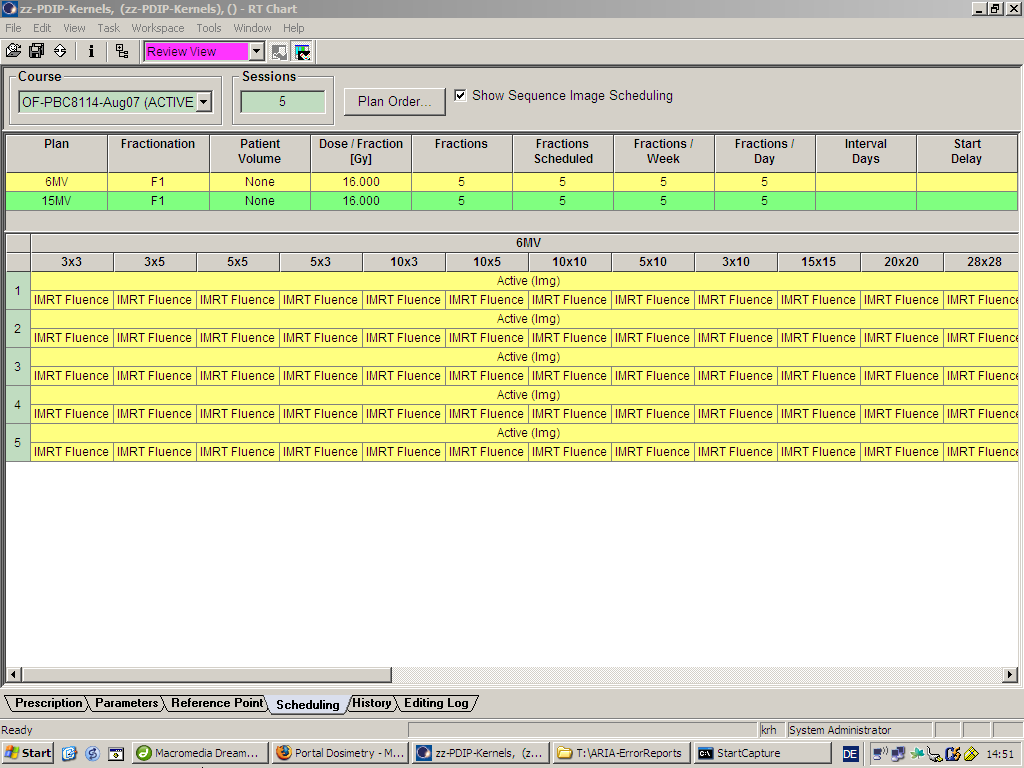
In Scheduling tab, add two sessions and fill in the plan. Add fluence images to the fields (that's the reason why you do all this).
In Reference Point tab, Treatment Approve the plan.
enter couch parameters
enter sequence images
treatment approval
Time Planner
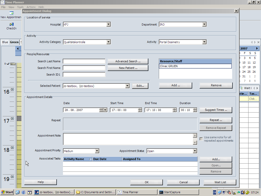
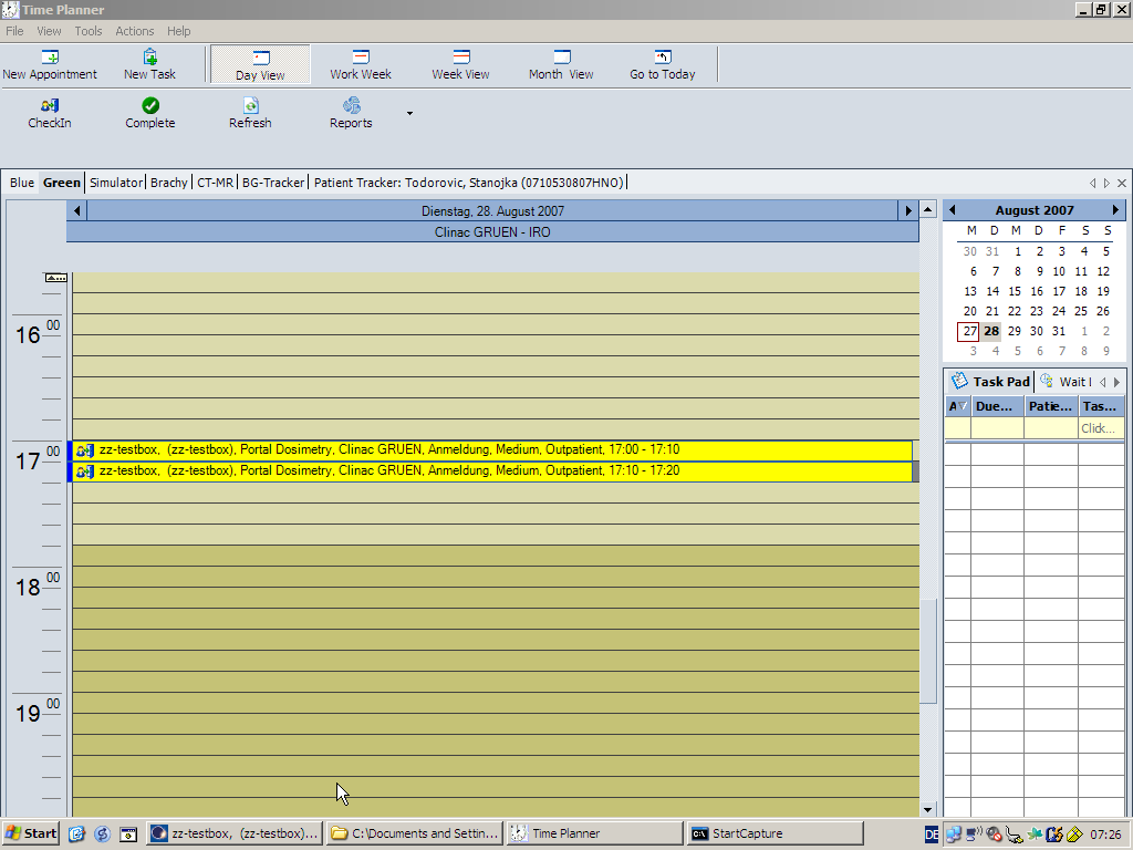
In Time Planner, give the Test patient two appointments on the linac and check him in.
check in patient
4D-Console
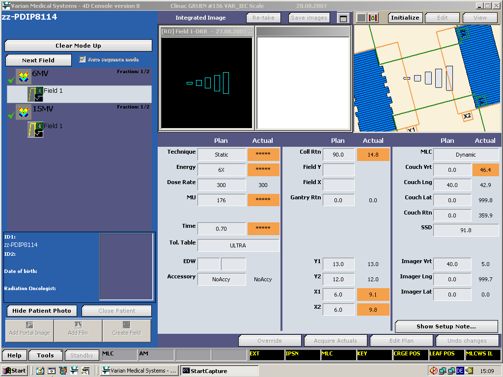
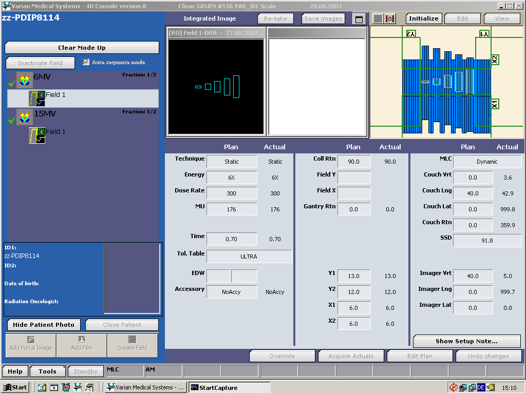
Treat the plans on the linac and acquire the images. Note: When the field is loaded in the first plan, the imager shall be positioned vertically at -5 cm (5 cm below isocenter). For the second plan, the imager shall be at -40 cm. Therefore, the Focus imager distances are 105 cm and 140 cm, respectively. Note: Lateral and longitudinal imager positions are always zero for Portal Dosimetry! (Note for the screenshots: I changed the name of the test patient from "zz-testbox" to "zz-PDIP8114").
ready to beam-on
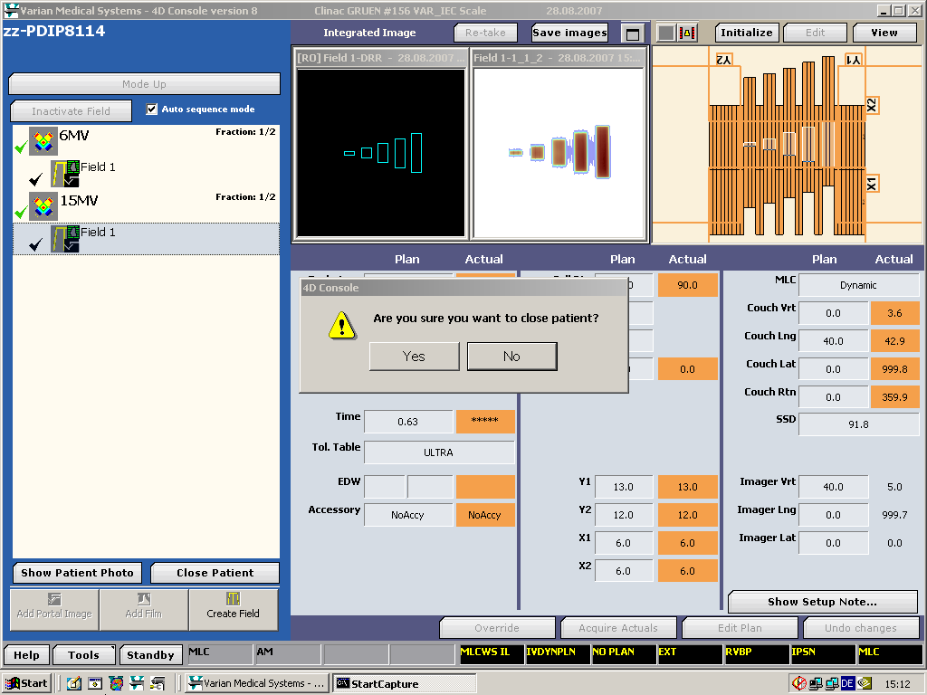
15 MV image at 105
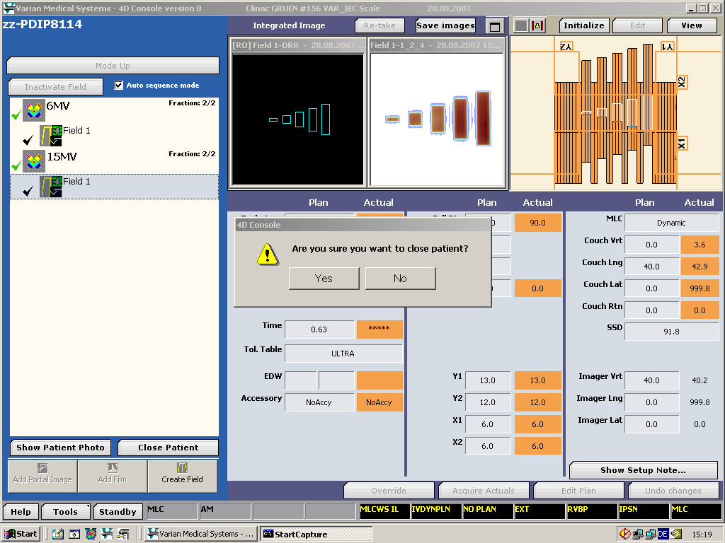
15 MV image at 140
Review Workspace
In Eclipse or Radiation Oncology, switch to Review (Dosimetry Review) and navigate to the sessions with the acquired images. Select the measured dose ( ![]() ) behind the image (expand the "+") and right-click "Eport dose to ASCII". Save it to a known location and name it "6MV_105cm.dxf". Export the second image and name it "6MV_140cm.dxf". Take care that the image named "105cm" is really the one acquired at 105 cm distance from focus! Here are some test images for 6 MV and 15 MV. Use them at your own risk.
) behind the image (expand the "+") and right-click "Eport dose to ASCII". Save it to a known location and name it "6MV_105cm.dxf". Export the second image and name it "6MV_140cm.dxf". Take care that the image named "105cm" is really the one acquired at 105 cm distance from focus! Here are some test images for 6 MV and 15 MV. Use them at your own risk.
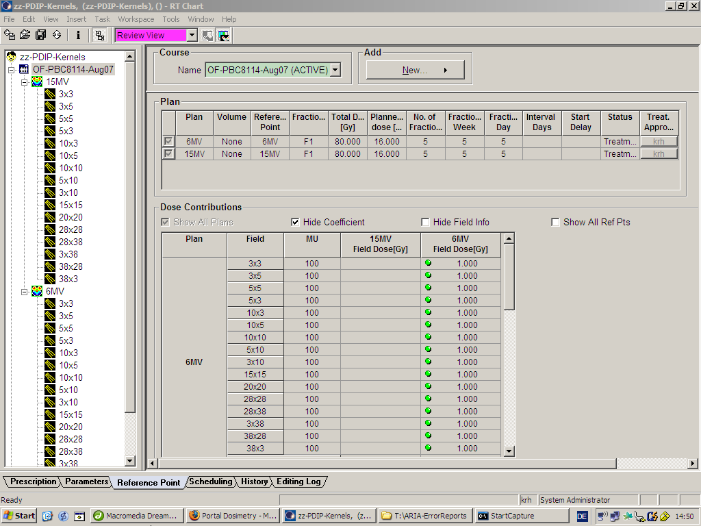
For the output factor measurements, prepare another test patient, this time in RT-Chart alone.
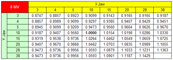
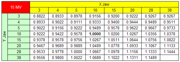
For each field of the test plan, an image is acquired. The center pixel value of each field with reference of the center pixel value of the 10x10 field is taken as the output factor.
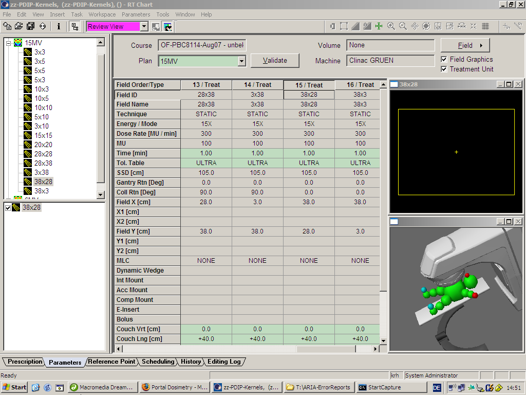
Note that some fields with 38 cm require collimator rotation because the imager orientation is landscape (40x30 cm). It does not make a difference whether the majority of fields (which fit on the detector) have collimator rotated to 90° or are at 0°. But for some fields the collimator has to be rotated, otherwise the output factor table cannot be filled completely.
It is recommended, but not required, to measure all (X,Y)-combinations of the sizes 3, 5, 10, 15, 20, 28, 38cm, except for (38x38), which is not possible. This would give 48 fields per energy. The test patient in the screenshots only has 16 fields.
The following tables show our output factors for 6 MV and 15 MV, measured with 300 MU/min at 105 cm on an IDU11 detector with 50 MU per image, evaluated in Dosimetry Workspace (Point Dose in the field center). Collimator was at 0° for most fields, and rotated to 90° for Y=38 fields.
plan scheduling
sequence images
collimator rotation for longest fields