Results (1)
CT Scan
The OP's "feet" of the 90° OP/OD tandem setup produced rather strong streak artefacts at the proximal and distal end due to the feet's metal screws. The first and last chamber rows of the OD are affected.
Compared to the S29, the material of the OD is of much higher density, leading to increased HU numbers: we measured an average of 1100 HU in the detector's back plane, over a large ROI (see screenshot). This is not a problem per se, as long as the heterogeneity correction of the TPS is working properly, or the OD is masked for dose calculation.
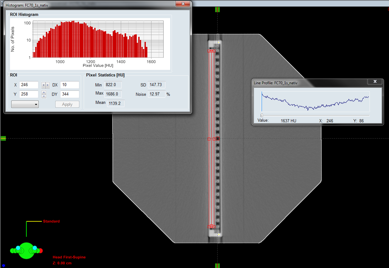
Fig.6: KFJ scan of the OD/OP-tandem in the 90° orientation.)
Also problematic for the accuracy of dose calculation on unmasked CT scans could be the beam hardening effect of the CT: a HU line profile across the same ROI (from top to bottom in the screenshot) measures between 822 HU (lowest point) and over 1600 HU (at the beginning of the profile).
The side walls of the OD and the 5 mm thick front plate are made of the same high density material. The area density of the front plate has therefore increased from 0.6 g/cm2 for the S29 to 0.8 g/cm2 for the OD.
Post-Processing and Contouring
The automatically generated BODY structure had to be corrected at the lateral edges of the OD. Because the OD is made of denser material than the S29, artefacts at the lateral edges of the OD "cancel out" the polystyrene phantom material, which affects the automatic BODY segmentation in Eclipse. At these locations, the BODY outline had to be restored manually.
If the OP is put directly on the carbon CT overlay during the CT scan (not on its "feet"), the phantom's bottom is in direct contact with the overlay. This shifts the BODY outline a little bit (2 mm in our case) into the overlay during the automatic BODY segmentation process. This part of the BODY outline has to be cropped during post-processing, otherwise a false SSD (83.8 cm instead of 84.0 cm, see below) and a dose error of up to 0.5% for fields at gantry 180° will result.
For the phantom sides which are undisturbed, we expected the phantom diameter of 32 cm to be exactly reproduced on the CT images. However, in Eclipse we measured a diameter of 31.8 cm between opposing undisturbed phantom surfaces. This means that our -350 HU threshold for the BODY generation is a little too high and does not reproduce the real dimensions of physical phantoms like the OP. Changing the HU threshold to -550 HU would give the correct size of the BODY outline (32 cm).
Shift between OD center and OP center
We visually determined the chamber center as it appears on the CT images ("apparent chamber center"), and measured distances from this point (marked as "Iso" in the screenshot) to the phantom surface.
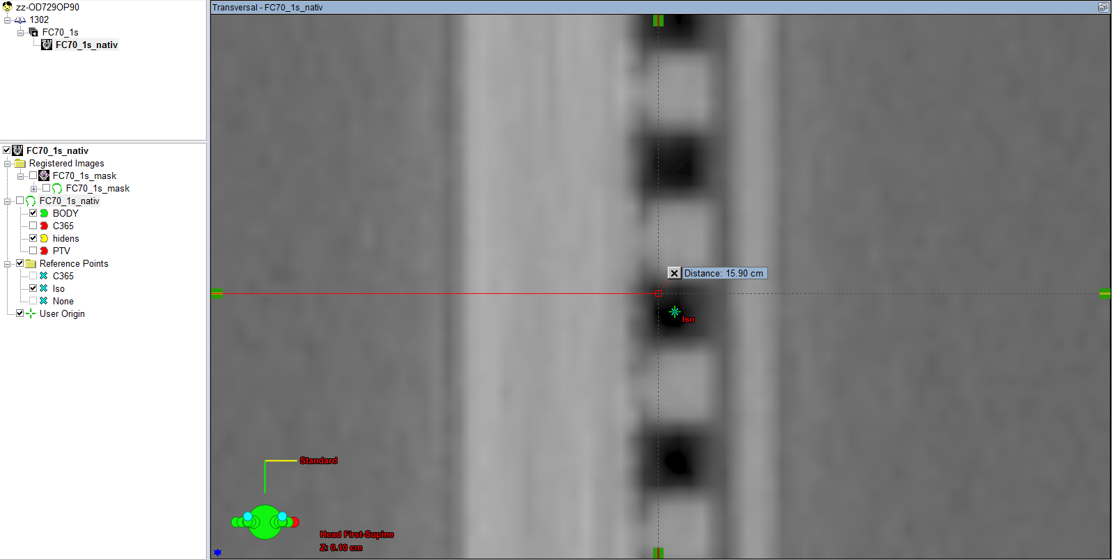
(Fig.7: The geometric center of the OP is not in the chamber center.)
We found that the central plane of the OD (through the apparent chamber center) does not coincide with the central plane of the OP (phantom center). If the field is aligned with the phantom center in Eclipse, the field isocenter on the CT image is therefore closer to the backplane of the OD by about 1 mm.
On the other hand, if the field isocenter is aligned with the chamber center (with the OD in the vertical orientation), Eclipse displays an SSD of 84.2 cm for beams entering from the front (gantry 90°), and 84.0 cm for beams entering from the back (gantry 270°).
We think the latter is the correct setup, for symmetry reasons. We define the plane through the apparent chamber center as the reference plane. This is also the dose plane we export from Eclipse. If the OD is in horizontal orientation, the correct SSDs in Eclipse are 84.1 cm to the sides (edges of OD), 84.2 cm on top (upstream) and 84.0 cm at the bottom (without couch, of course).
When the phantom is set up on the linac, the OP's grooves which run around the phantom (marking the phantom's symmetry planes) are usually aligned with the room lasers. Since the grooves mark the phantom center, not the chamber center, this leads to field isocenters which are shifted towards the OD backplane by 1 mm. We also use the grooves for aligning, but finally apply a 1 mm phantom shift downstream (so that the OD's entrance surface moves away from focus). This moves the isocenter upstream, into the chamber center. The SSD on the linac changes from 84.0 cm to 84.1 cm.
We do not know whether this shift between phantom and Array is intended or not.
The mechanical play of the OD inside the OP is still the same as for the S29 (outer dimensions are identical): in horizontal orientation, we measure a 1 mm air gap above the OD. In contrast to the S29, this is hardly visible on CT images, due to the much higher HU values of the OD housing, which obscures the gap. On the sides of the OD, we insert two cardboard strips. This removes any lateral play of the OD inside the OP.
Simple Opposing Fields - Unmasked Structure Set "native"- AAA
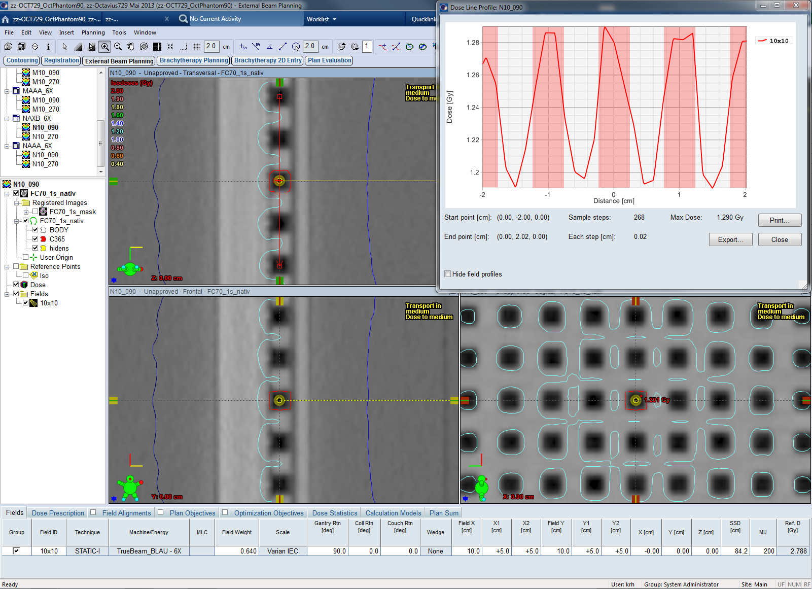
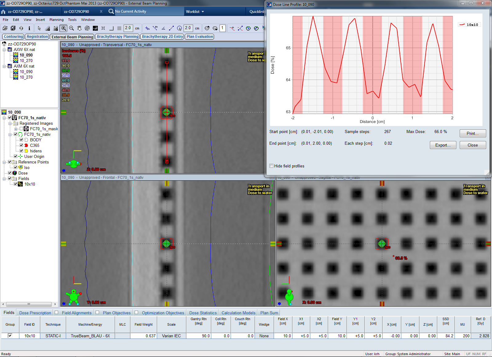
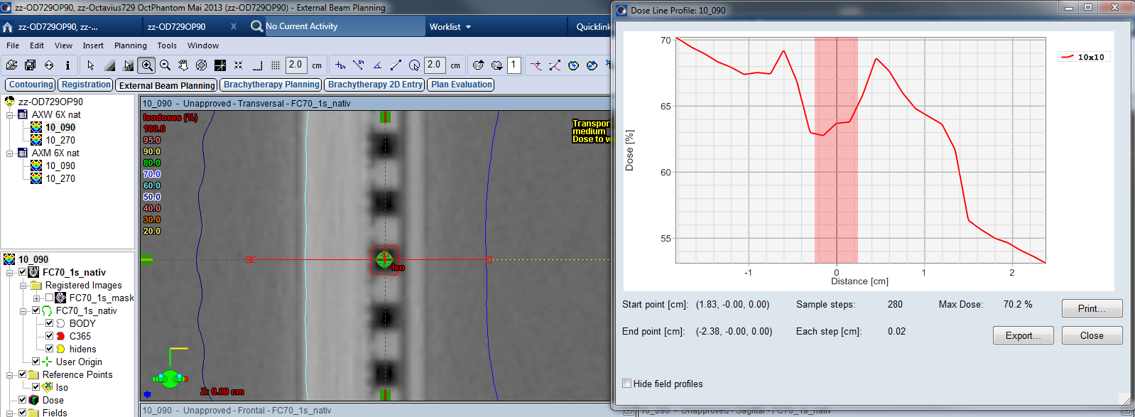
With the "native" (unmasked) OD, a dose profile across the ion chambers (zero point at CAX, beam entering from the right) shows peaks and valleys, with the highest dose values in the dense material between the cavities. In this and the following screenshots, the air-filled chamber volume is shaded in red:
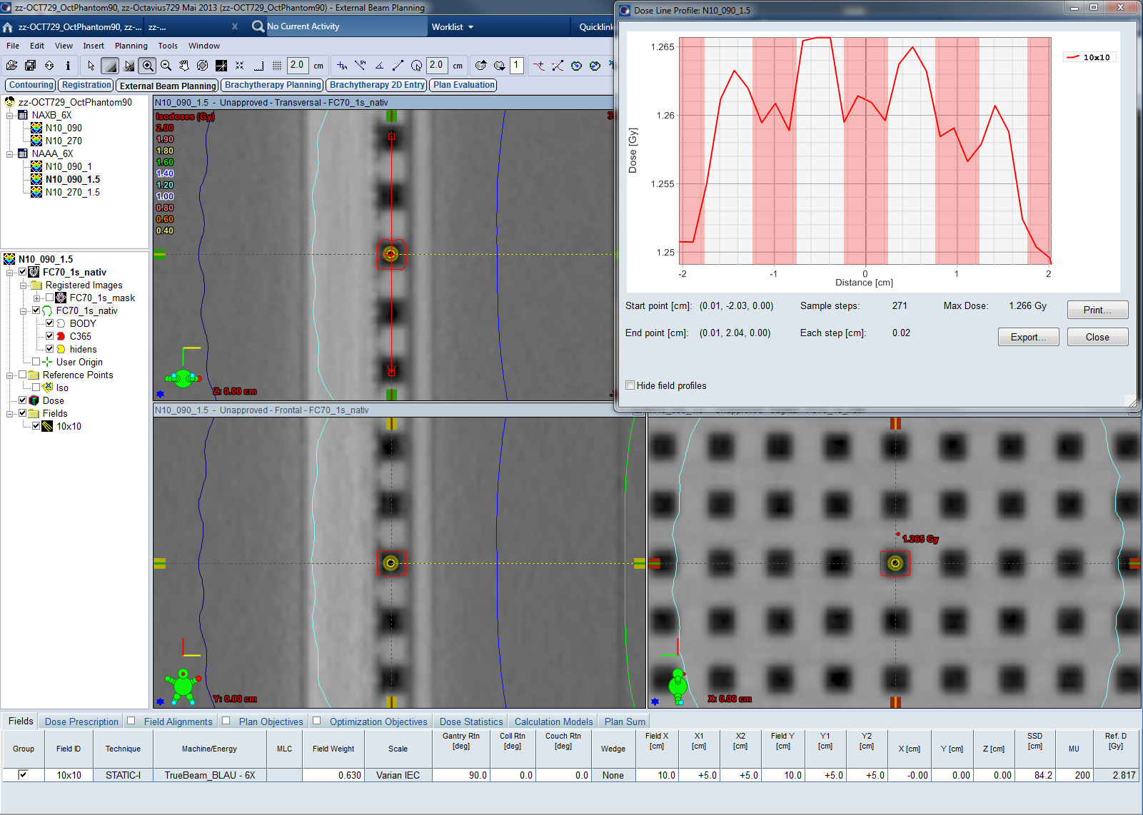
(Fig.8: AAA calculated cross-chamber profile. Calc grid size 1.5 mm.)
Suspecting a calculation grid effect, we reduced the grid size to 1 mm. Surprisingly, peaks and valleys switch position (!): dose peaks now coincide with the chamber cavities, whereas the valleys are between the chambers:
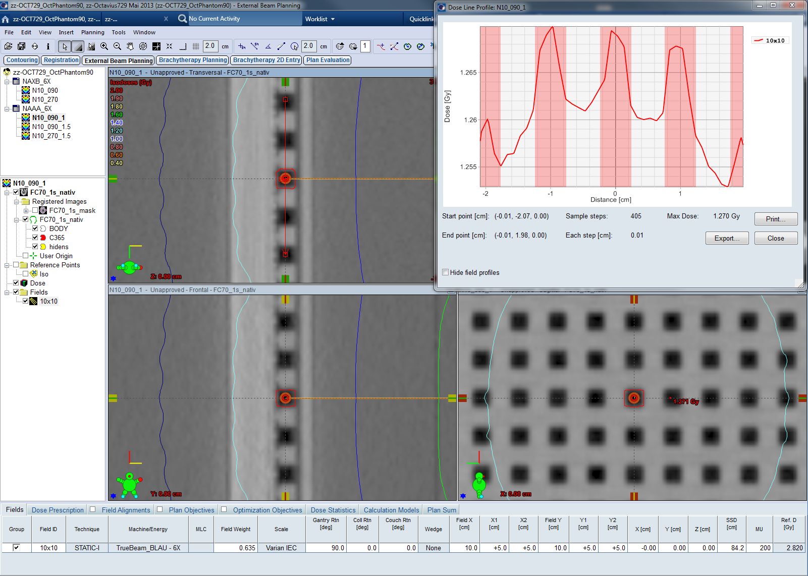
(Fig.9: : AAA calculated cross-chamber profile. Calc grid size 1.0 mm.)
This calculation grid effect can change a cross-calibration factor by 2%. The following screenshot shows a comparison of two dose planes through the chamber centers (central region of a 6 MV, 15 x 15 cm field), calculated with AAA11031 and different grid size. Top left is 1.0 mm grid, bottom left is 2.5 mm grid (our clinical default setting). Dose was calculated on the native scan of the OD/OP tandem. Local dose difference inside the chambers is up to 2%:
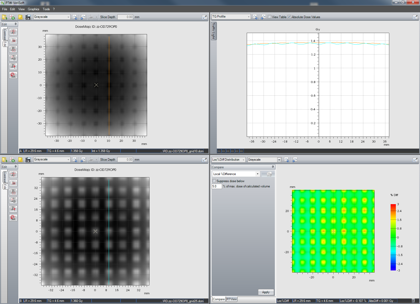
The conclusion is that one has to be very cautious when using dose planes calculated with AAA on native scans!
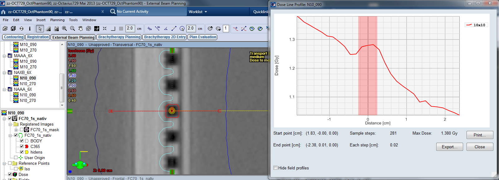
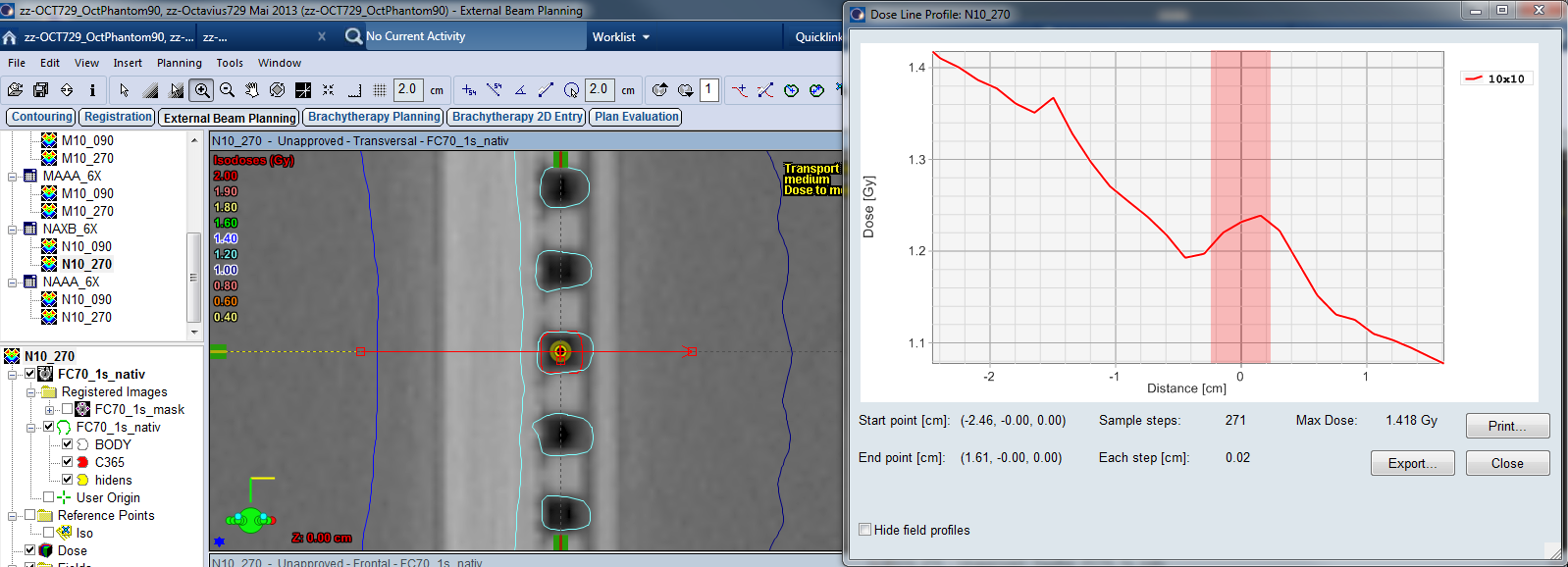
Due to the OD's asymmetric construction (chamber matrix closer to the surface, backplane made of high density material), depth dose curves measured through C365 are not expected to be symmetric.
If the beam enters the OD through the front plate (from right to left), it looks like this:
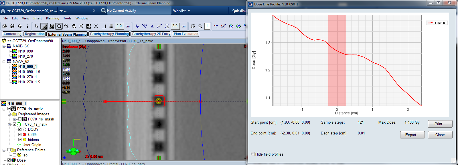
(Fig.10: AAA calculated depth-dose curve - normal beam incidence.)
An opposing beam through the OD's back plane (gantry 270° in the 90° setup) has to cross 10 mm of Vetronit and 2 mm of PCB before it reaches the chambers:
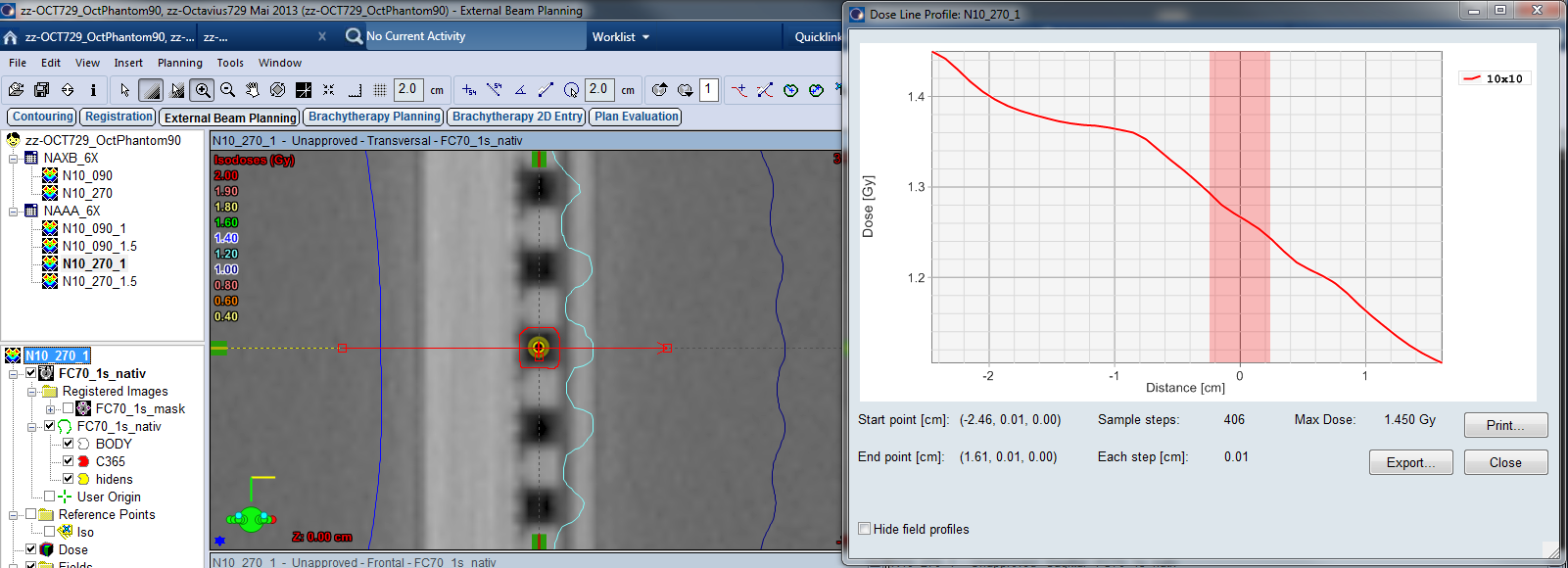
(Fig11: : AAA calculated depth-dose curve - reverse beam incidence.)
The zero point of the profile is positioned at isocenter (chamber center). This means that the chamber extends 2.5 mm upstream and 2.5 mm downstream.
Simple Opposing Fields - Structure Set "native" - AcurosXB "Dose to Medium"
In the calculated dose profile and using a grid size of 1.5 mm, AXM displays strong dose "waves" with an amplitude of over 7%:
(Fig.12: AXM calculated cross-chamber profile. Calc grid size 1.5 mm.)
Dose peaks are inside the chambers, whereas the valleys are in the higher density material between the chambers. This is in agreement with the 1 mm AAA calculation.
Similar to the crossplane profile, the AXM calculated depth dose shows much higher local gradients than the AAA calculation. Dose increases when the beam enters the chamber cavity:
(Fig.13: AXM calculated depth-dose curve - normal beam incidence.)
(Fig.14: AXM calculated depth-dose curve - reverse beam incidence.)
The "bump" around zero depth is the chamber volume. In beam direction, the dose max is always behind the chamber center.
Inside the segmented C365 chamber volume, the difference between max dose and min dose is 4.6% for the gantry 90° field, and 4.3% for the gantry 270° field.
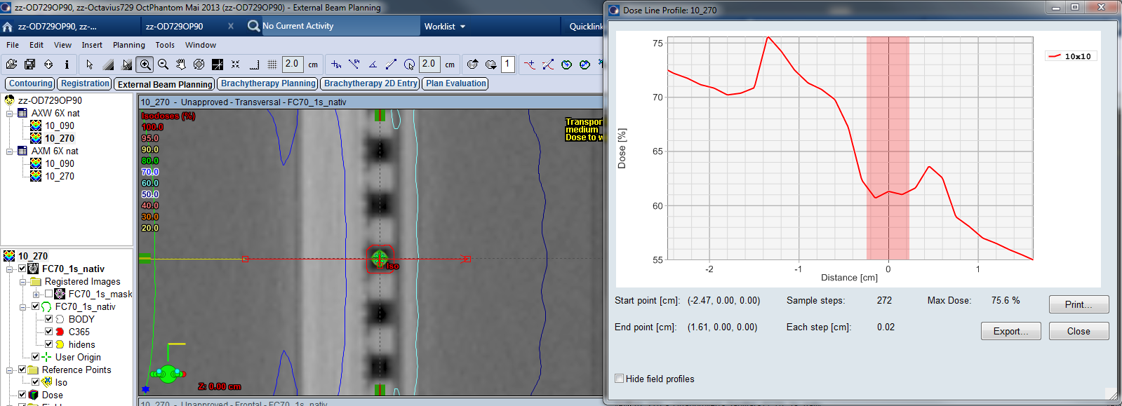
Simple Opposing Fields - Structure Set "native" - AcurosXB "Dose to Water"
In the "dose to water" crossplane profiles, the locations of peaks and valleys have switched position with respect to the AXM calculations. Now the air-filled cavities have lower dose, and the dose peaks are between the chambers. The amplitude of the oscillations has dropped to about 3.5%:
(Fig.15: AXW calculated cross-chamber profile. Calc grid size 1.5 mm.)
A similar phenomenon was observed for AAA, but this time it is not a grid effect: AXM and AXB calculations both used the same grid size of 1.5 mm.
Consequently, where there was a bump in the AXM depth dose curve, the AXW depth dose curve shows a dose depression inside the chamber cavity:
(Fig.16: AXW calculated depth-dose curve - normal beam incidence.)
(Fig.17: AXW calculated depth-dose curve - reverse beam incidence.)
From this planning study one can already guess that due to the inhomogeneities of the OD, it will not be easy to get good verification results with native CT scans of the OD/OP tandem, especially if the dose calculation algorithm is AXM or AXW.