Analysis
of Dynamic MLC Files
 Visualizing a dynamic
sliding MLC window in a single image can be tricky. As the sliding window changes
its outline constantly, the width of the field opening defined by each leaf
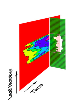
pair is a function of time. In this composite image the colour plot shows the
sliding window width for each leaf pair and shape as a function of time, encoded
in colors. Red means that the actual field opening is less than 1 cm, yellow
means 1-2 cm and so on. The largest gap is between 5 and 6 cm wide (purple).
Visualizing a dynamic
sliding MLC window in a single image can be tricky. As the sliding window changes
its outline constantly, the width of the field opening defined by each leaf
pair is a function of time. In this composite image the colour plot shows the
sliding window width for each leaf pair and shape as a function of time, encoded
in colors. Red means that the actual field opening is less than 1 cm, yellow
means 1-2 cm and so on. The largest gap is between 5 and 6 cm wide (purple).
The abscissa could also
be labelled with shape index, dose fraction or accumulated MUs - they all mean
the same thing. If the treatment is performed by beaming 250 MUs @ 600 MU/min
and the DMLC file has 200 shapes, a dose fraction of 0.65 is reached after 163
MUs or 16 seconds. After 16 seconds shape number 130 is reached. So far the
theory - if dose rate is not stable, things look different. But after all, this
plot shows how things should look like.
At the dose fraction of
0.65 (or after 16 seconds), a snapshot of the actual MLC shape 130 is also shown
standing perpendicular to the plot. The width of each leaf pair in the shape
is encoded in different colours in the Contour Plot at the position of the vertical
white line.
Calculation of Leaf Velocities
So far, there was not much
dynamics in the example. Further analysis of the DMLC file can be done by calculating
the leaf velocities of all leaves during the treatment. This should be done
to check the Leaf Motion Calculator's output. When the LMC performs its optimization,
it is aware of the physical speed limit of the leaves (here: 2.5 cm/s). When
analyzing the LMC output, no leaf should exceed this limit during the treatment.
For the velocity calculation, the simple equation s = v * t is taken, and a
constant velocity within a segment is assumed. This is also what happens on
the machine, since leaf speeds within a segment are constant. If the number
of MUs (250) and the dose rate (600MU/min) is taken from above, velocities in
cm/s can be calculated simply by taking the difference of leaf positions for
subsequent shapes and dividing this distance by the time it take to "beam"
from dose fraction i to dose fraction i+1.
Plots can be drawn for the
leaf velocities of leaf bank A and B (vA, vB), or the maximum of both (Max[vA,
vB]).
Dose rate modulations can occur as a result of
wrong user settings or bad mechanical parts (e.g., if a leaf motor draws too
much current as a result of increased friction). For instance, if CadPlan is
configured to perform dose dynamic treatments at 300 MU/min and the user selects
600 MU/min on the machine, such modulations may occur. Or, if the dynamic leaf
tolerance is reduced to a very small value, modulations of output are very likely
to be the result. But this does not mean that the dose applied to the patient
will be different! The resulting dose distribution will be the same, independent
of dose rate variations. This is guaranteed by the control mechanisms and was
already thoroughly investigated on our machines.
back to Medical Physics home