DYNALOG analysis using MATLAB®

DYNALOG Refresher

During delivery, the true and planned leaf positions are sampled by the MLC control computer every 50ms with a precision of 1/100 mm at MLC level (magnification factor for the Varian Standard-80 MLC is 1.96614).

This means that:

• If a DYNALOG file contains 900 records, delivery took 45 seconds.
• If a leaf position of 2500 is encountered, the leaf was 49.15 mm off central axis.

One field, many views

The following (hand-made) DMLC sequence shall serve as an example how different views can be retrieved from the DYNALOG files of the same treatment.

The logs of this treatment have code 042 in the zipped collection.

Leaf position ('pos.m')

Files A (right leaf bank) and B (left leaf bank) are analyzed separately.

Color represents leaf position or leaf deviation. Beam-holds are ignored (click all images to enlarge):

All leaf positions (A and B) now consistently increase from left to right (the B axis is reversed with respect to DYNLOGB).

Leaf gap ('gap.m')

Instead of looking at the A and B leaves separately, in this script the gap width of each leaf pair as a function of time is color encoded:

Fluence ('flu.m')

Beam-on information is crucial, but this was ignored so far. If a certain leaf is at the wrong position, it is no problem as long as beam is off. The Varian control system makes sure that beam pulses get delayed (no beam output) as soon as a leaf is off its planned trajectory. This happens within 100 ms.

The 'flu.m' script produces output that can be interpreted easily: it is more or less what you would get on film. Both axes represent distance, although it is a matter of scaling to get the aspect ratio right (we will ignore that).

Because the resolution is so high, be cautious when interpreting the error fluence map on the basis of the range of the colormap alone.

Only if a significant percentage of image pixels holds a certain color, the respective fluence error (as taken from the colormap) is valid.

We leave our doughnut and come to another example.

Slow leaf

When a field which is calculated for 300 MU/min is treated with 600 MU/min and there is a leaf whose motor needs replacement, one can observe the following (this was done without patient, of course):

'Huston, leaf pair 20 has a problem!'

(Note: in the MATLAB pcolor()-plots, the leaf numbers are aligned with the lower edge of the leaf pairs.)

Position analysis reveals that the motor of A-20 should be replaced:

Also the gap error (up to -5 mm) is quite significant. The right A-leaf lags behind, which narrows the gap:

For completeness here are the planned and true fluences:

We want to come back to the topic of 2001, where we described some ways of analyzing sliding window (DMLC-) treatments on our Varian machines (Clinac 2300C/D with 80-leaf MLC). This can be used for pre-treatment fluence verification and daily treatment monitoring - a software alternative to hardware devices like DAVID or Compass.

Since MATLAB has become the standard of technical computing, we want to review the DMLC topic by using this tool.

Starter package

There are four very simple MATLAB scripts:

• Position analysis ('pos.m')
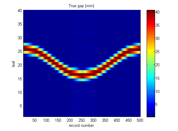
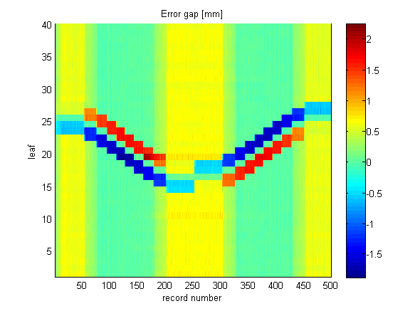
• Gap analysis ('gap.m')
• Velocity analysis ('vel.m')
• Fluence analysis ('flu.m')

All scripts are heavily commented. It should become clear what they do after reading the comments in the source code.

Principle of fluence computation

In principle, photons are getting through the MLC (hitting some virtual film) whenever

• a leaf pair is open (locally exposing the film to the beam)
• current dose rate is larger than zero.

In the 'flu.m' script, the difference in MU counter (1st column of the log files) from one record to the next is interpreted as current dose rate. Every 50 ms, the value of each exposed pixel in the fluence matrices 'fp' (planned fluence) and 'ft' (true fluence) are increased by the current dose rate. This is how the fluence maps build up.

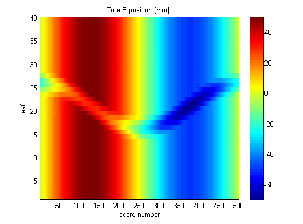
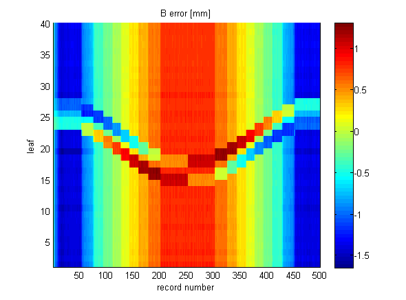
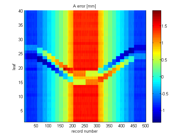
Note that the fluence script uses a distance scale which is different from the position/gap/velocity scripts. The fluence script use the raw scale for the horizontal axis (the direction of leaf movement). In the other scripts distance is plotted as a function of time. The distance is in terms of [mm] at isocenter. The time (horizontal axis) is in terms of record number (20 records representing 1 second of delivery - see sidebar).

For the sake of simplicity, we ignore the jaws. Leaf pairs that will not move during a treatment are always 'parked' under the jaws. Since we ignore this, in our fluence computation closed leaf pairs 'burn a hole' into film. In the 'flu.m' skript, we therefore crop the fluence maps: 2 mm on the left border (where the closed leaf pairs are usually parked) are cut away.

Here is a ZIP of some sample DYNALOG files to play around with. The first line in each file is already removed (see comment in scripts), so they can be loaded without prior editing.

Clinical example

On our old machines with their old MLC controller running under DOS, it is uncommon to save logfiles after real patient treatments¹. After saving the files, one has to exit the MLC controller software to get to DOS, ZIP the logs, copy them to floppy (here the doit script helps a lot), and reinitialize the MLC. This is unacceptable in a busy department.

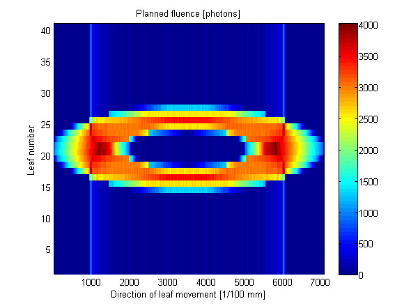
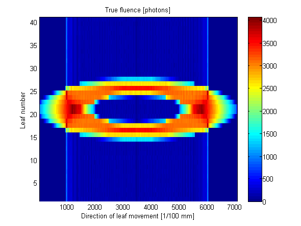
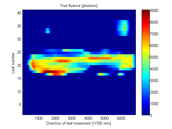
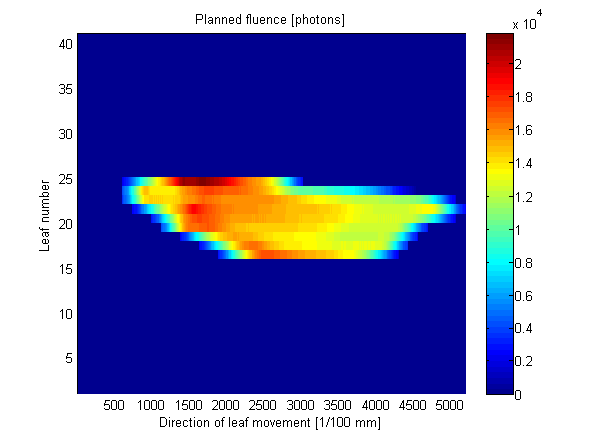
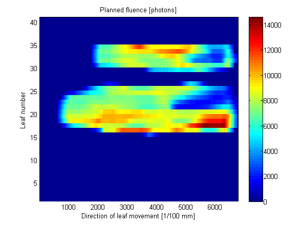
Here is one example of a typical lateral prostate IMRT field. Planned and true fluence are visually indistinguishable:

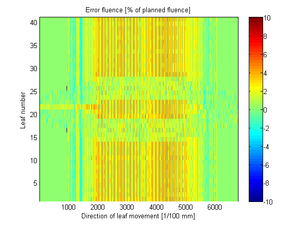
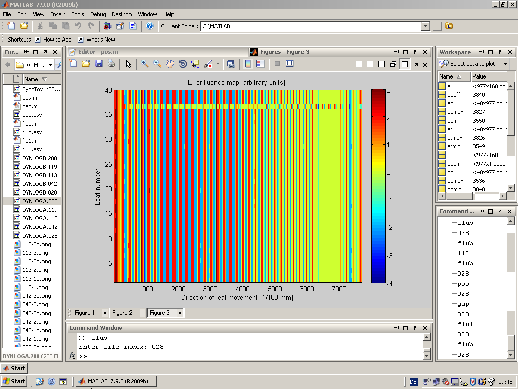
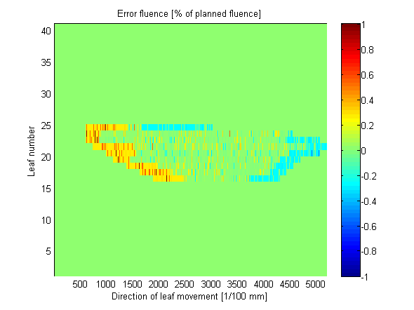
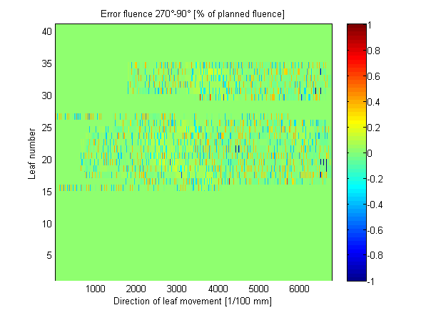
The colormap of the error fluence was already adapted, so that a noticeable fraction of image pixels show up. Compared to the planned fluence, the maximum error is around 1%:

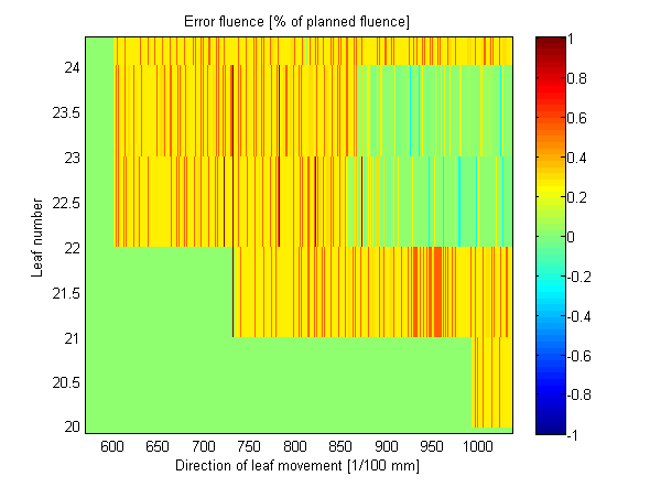
The zoom gives an idea of the high resolution. The stripes with the higher error are extremely small. Yellow dominates. This corresponds to a local fluence error of 0.3-0.4%:

Gravity tests

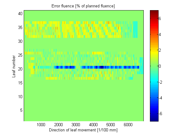
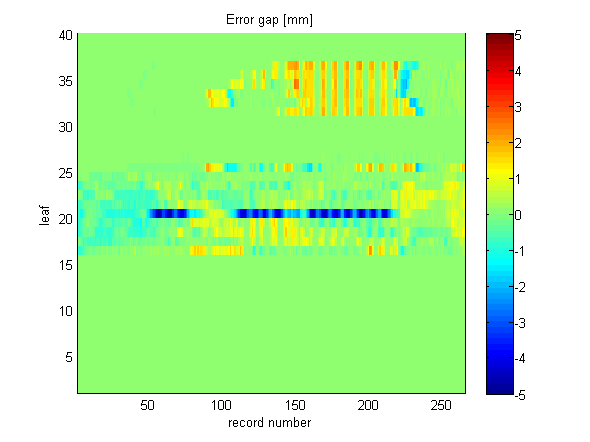
If there are gravity effects, they could be visible on the logs as well. In the following example, a field was treated at Gantry angles 0°, 90° and 270°. At 90° leaves are allowed to go 'down', at 270° they are forced to go 'up'. This is how the planned fluence looks like:

One can use the 'flu.m' script for the 90° side, save away the true fluence ft90 to a new variable, (comment out the 'clear' command in the first line of the script, otherwise ft90 will be gone!) evaluate the 270° side, and calculate the difference of the true fluences ft270 - ft90. The resulting plot suggest that there is no dependence on gravity:

¹ Of course one can always generate logfiles without the patient on the table!

back to Medical Physics home