

In a modern Radiotherapy department, 3D- treatment planning is typically based on CT-images. Depending on the dose calculation algorithm used, it is either necessary to convert the scanner's Hounsfield Units (HU) to relative electron density (EDens) or to mass density (MDens). The former applies to algorithms like AAA, the latter to algoritms like AcurosXB or eMC, which perform material mapping.
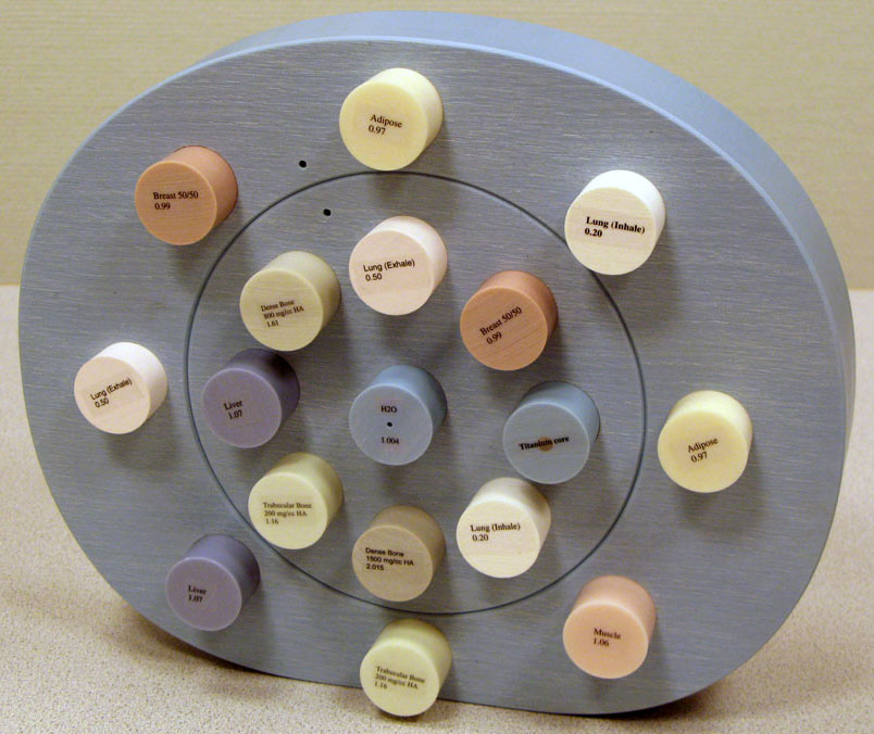
The HU to EDens and HU to MDens conversions are accomplished with calibration curves, which are determined with the help of a certain phantom (see sidebar). These curves link the HU values measured on the scanner to known EDens or MDens values of the phantom inserts, which are provided by the manufacturer of the phantom.
In Eclipse, only one calibration curve of each type may be defined per scanner. For accurate dose planning, the scanner's HU-distributions should therefore ideally be:
- independent of energy (the scanner's kV setting)
- independent of other scanner settings like collimation, reconstruction kernel, single slice or helical scan, image filters, ...
- free of artefacts (visible artefacts mean wrong HU!)
- independent of data collection diameter (Calib-FOV)
- independent of the size of the scanned object, for the same Calib-FOV.
The last requirement is specific for the radiotherapy treatment planning process. On a diagnostic scan, it is usually possible to match the Calib-FOV to the size of the object. For a head scan, a small FOV is normally used. On a treatment planning scan, it is necessary to include all immobilization devices on the image which might be penetrated by the therapy beam. In a head and neck case, this includes carbon base plates and head rests, which are often as wide as the therapy couch itself (> 500 mm). A large FOV has to be chosen for such a scan, otherwise these parts would not be imaged, and attenuation of the treatment beam could not be properly accounted for.
Choosing a large FOV in this case also means that the main object (the patient's head or neck) is much smaller than the selected FOV (e.g., 700 mm). This leads to the paradox situation that for the smallest scanned object (head), the largest FOV has to be used, while for a pelvic scan smaller FOVs are sufficient.
Materials and Methods
After proper HU calibration by Toshiba field service engineers, we scanned the "Head" and "Pelvis" electron density phantom, to test the above-mentioned dependencies and to finally generate calibration curves for Eclipse.
In all scans (which were performed in helical mode), the phantoms were placed on the UCT overlay, which means that the influence of the carbon couchtop is included in the calibration curves.
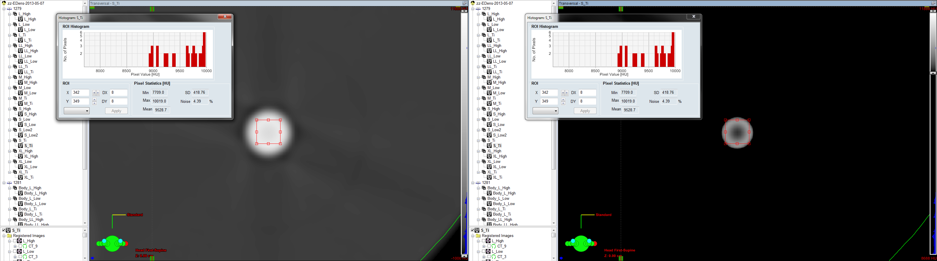
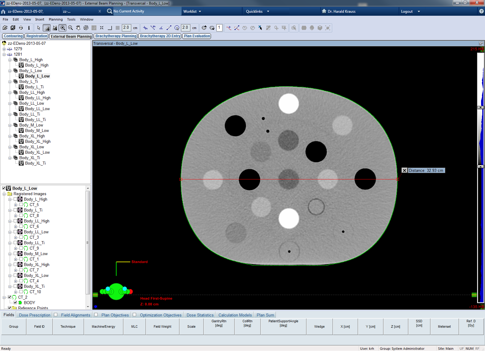
The material inserts were more or less randomly placed in the phantom. After transfer to Eclipse, in the central CT slice of the phantom (Z: 0.00 cm) histograms of the materials were measured,
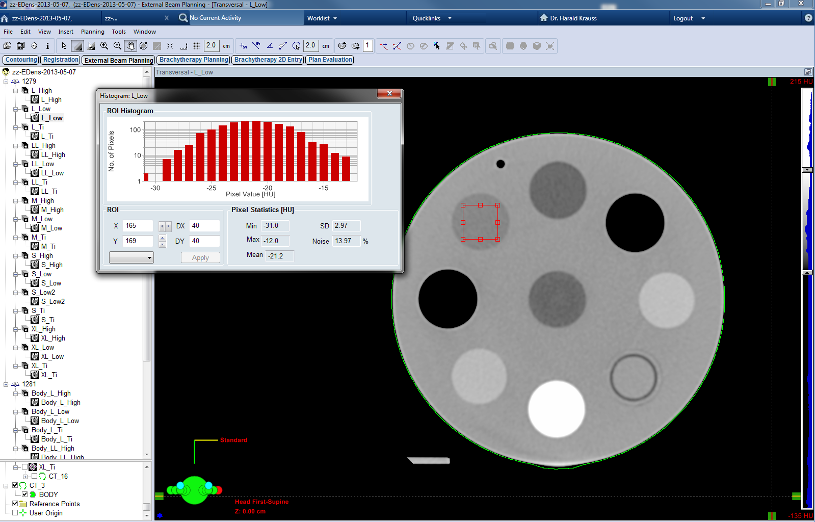
and the mean HU value determined for each insert (here: -21.2 HU for Breast).
To reduce the impact of artefacts on the final calibration curve, Head and Body phantom were scanned in three different setups:
- The "Low" density setup only contained plugs with densities up to B200, but not higher. Only the densities from Lung Inhale up to B200 were evaluated and used for the calibration curve.
- In the "High" density setup, the low density lung inserts were replaced by the second B200, the B800 and the B1500 plugs. In these scans, only the histograms for the bone inserts B800 and B1500 were evaluated.
- In a third "Titanium" setup, the water syringe was replaced by the Titanium plug. Only this plug was evaluated.
The "Low", "High", and "Titanium" setups are shown from left to right for the "Head" phantom:
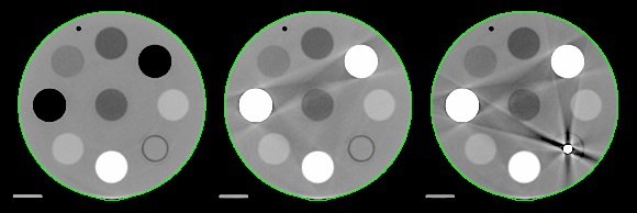
(Scan settings: 120 kV, 300 mA, 1 s, 1.0 x 16, Image thickness 2 mm, TCOT, FC17, QDS+)
From data of the three setups, we generated a composite calibration curve in the range from Lung Inhale to Titanium. At the lower end of the calibration curve, an "Air" point (-1000 HU) was added without measurement.
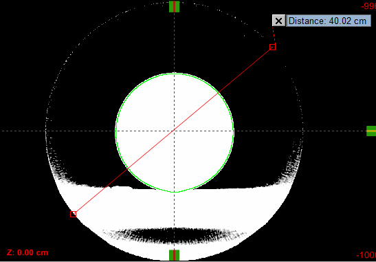
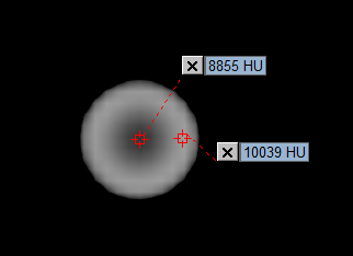
The Titanium point itself has a large uncertainty. Although the rod has only 1/4", the scan shows strong beam hardening inside the rod, which leads to large HU differences between the center and the periphery of the rod. Eclipse does not allow circular ROIs, which makes it even harder to determine meaningful values on circular structures:
(Beam hardening inside Titanium rod. HU-display left: -1000 to 11800, right: 8688 to 11800)
This makes it hard to define a reliable Titanium point for the calibration curve. We used a mean value which was taken from the histogram of a small square ROI, similar to the above screenshot. However, in this example, a HU point measurement gives 8855 HU on the rod's axis but 10039 HU in the rod's periphery.
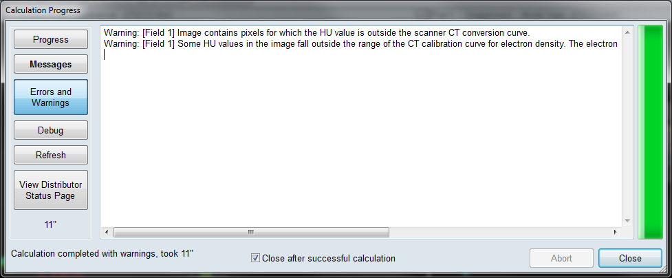
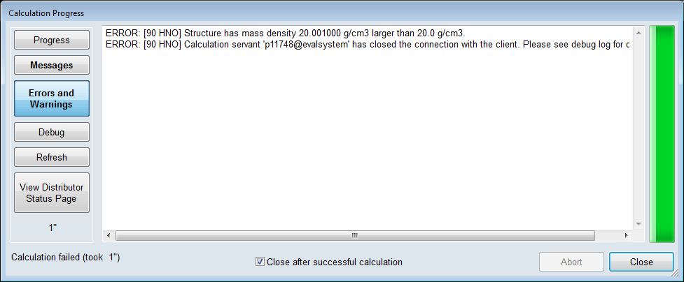
Beyond Titanium, an "artificial" calibration point was defined at very high MU (29768 HU for the EDens curve), to reduce the occurence of "outside range" warnings in Eclipse dose calculation, see sidebar.
Results
Dependence of HU on Energy (kV)
The highest possible kV setting on the AquilionLB is 135 kV. Energies lower than 120 kV had already been deactivated during installation of the scanner.
When the Titanium rod inside the Body phantom is scanned with 135 kV instead of 120 kV, the HU of Titanium are lower by about 1000 units (7800 HU vs. 8800 HU for 120 kV). The higher the density of the material, the larger the difference between the two energy settings. For B200, the difference is about 20 HU, materials with densities below B200 show no effect.
This makes it impossible to construct a single electron density calibration curve for the TPS which works evenly well for both kV settings (if one does not want to calculate an "averaged" curve over both energies, of course).
A definite calibration curve can only work for one energy. As conclusion, we have chosen to deactivate the 135 kV setting on the AquilionLB, so that it can neither be used in scan presets, nor by manual selection. Scanning is now only possible with 120 kV.
Dependence of HU on Calib-FOV: Head Phantom
The dependence of HU on the size of the Calib-FOV was first assessed for the "Head" phantom. With its 18 cm diameter, the Head phantom fits inside all five available Calib-FOVs from 240 mm (S) to 700 mm (XL). The phantom was scanned with a constant Display-FOV of 240 mm, which gives equal pixel size for all scans, and large evaluation ROIs (40 x 40 px for the standard inserts, 30 x 30 px for the water syringe, and 8 x 8 px for Titanium). The image size as transferred to the TPS is always 512 x 512 px, therefore the same object will be covered by more pixels, if the Display-FOV is small.
With three different setups ( "Low", "High", and "Titanium"), this gives a total of 15 scans for the Head phantom.
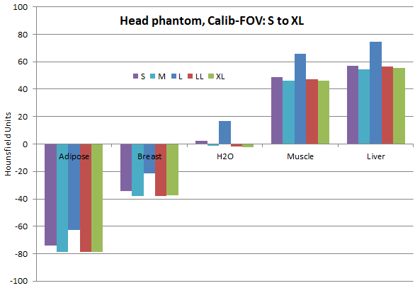
If one looks at the materials with densities close to water (Adipose to Liver), one can immediately see that there is something wrong with the "L" Calib-FOV (400 mm): HU numbers are consistently higher than for the smaller (S, M) and the larger (LL, XL) FOVs. Water in L for instance is not 0 HU, but 16.7 HU:
If the LL data are used as reference (rather arbitrarily, but LL is the standard FOV at our institute), the HU differences for the Head phantom and the other Calib-FOVs can be displayed for a larger density range (Lung Inhale to Titanium is here):
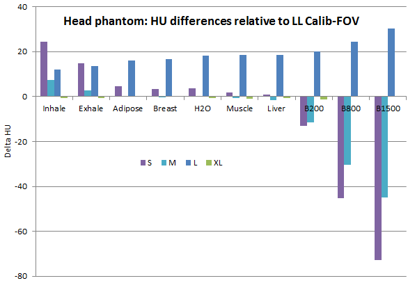
As conclusion, the L Calib-FOV should be deactivated on the AquilionLB or at least not used, because there is a systematic HU shift to higher numbers, even after proper HU calibration by Toshiba engineers.
For radiotherapy planning purposes, all Calib-FOVs smaller than L are irrelevant anyway, since they are too small. This means that for constructing the calibration curves, only scans with the LL and XL Calib-FOV should be used.
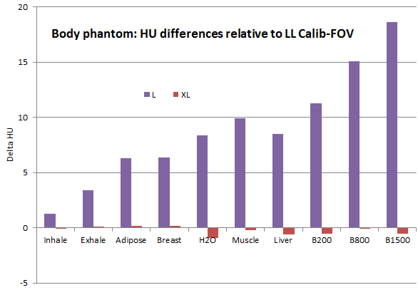
Dependence of HU on Calib-FOV: Body Phantom
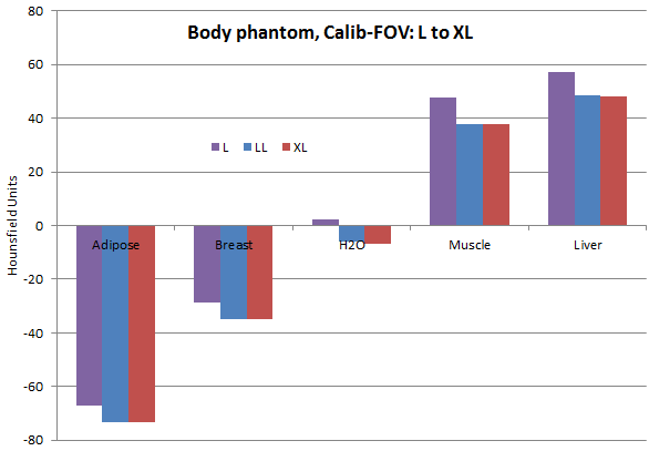
The larger diameter of the Body phantom of about 33 cm allows scanning with the L to XL Calib-FOV. Display-FOV was set to 400 mm. This results in ROI sizes of 24 x24 px for the standard plugs, 18 x 18 px for the syringe and 5 x 5 px for Titanium. The systematic shift of the L Calib-FOV to higher HU values also exists for the Body phantom.
If LL is again used as reference, a plot of the Lung Inhale to Bone 1500 range reveals that LL and XL give nearly the same HU. This makes them equally suitable for treatment planning purposes.
Dependence of HU on Phantom Size
We compared the HU of "Head" and "Body" scans in the following way: in the Head phantom, only the 8 plugs in the outer ring were evaluated, not the plug in the center (which is another Adipose plug). When the whole Head phantom is put inside the ring of the Body phantom,

the evaluated plugs remain the same. Inside the Body phantom, they are now at an "average depth" (neither close to surface, nor in the center). However, for the construction of a calibration curve, it makes sense to put a certain plug at as many phantom locations as possible, to acheive an averaging effect (HU in the center and the periphery are never the same).
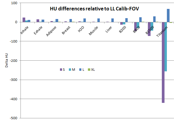
If one uses the HU values from the Body scan (mean values of LL and XL) as reference and plots the HU differences of the Head scans relative to this reference, one gets the following:
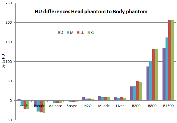
In other words: a B1500 plug in the Head phantom has 200 HU more than in the Body phantom, for the same Calib-FOV. On the other hand, low density materials in the Head phantom have lower HU than in the Body phantom.
Now this is a major problem when it comes to generating a good calibration curve for the TPS. The head and neck anatomy is full of bones, so when a TPS calibration curve would be generated on the basis of Body scans alone, the HU of bones in head and neck patients would be overestimated.
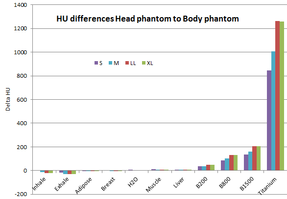
The Titanium values are not even shown here, since the large differences for Titanium would squeeze the vertical axis. Titanium inside the Body phantom gives about 8800 HU, whereas in the Head phantom, the same rod gives 10000 HU.
Dependence of HU on Reconstruction Kernel
The typical kernels like FC17, FC13, or the technical FC70 produce consistent HU values. There exist kernels which are known to shift HU, but these kernels are marked by Toshiba to be used with caution (not for treatment planning).
Construction of the final calibration curves
From the dependencies analysed it is clear that with the AquilionLB it is not possible to construct EDens and MDens calibration curves that work equally well for both head and body patients. Although some factors which have an impact on HU have been ruled out (deactivation of 135 kV and L Calib-FOV, restriction to only certain reconstruction kernels like FC17 or FC13), the biggest problem is the dependence of HU on the size of the scanned object, for densities other than water.
Thus, one can only compute "average" HU numbers for the different material plugs, potentially using weighting factors according to patient numbers (if 40% of all patients get head scans but 60% get body scans, a point can be made of putting a higher weight on the Body HU values).
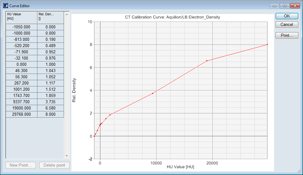
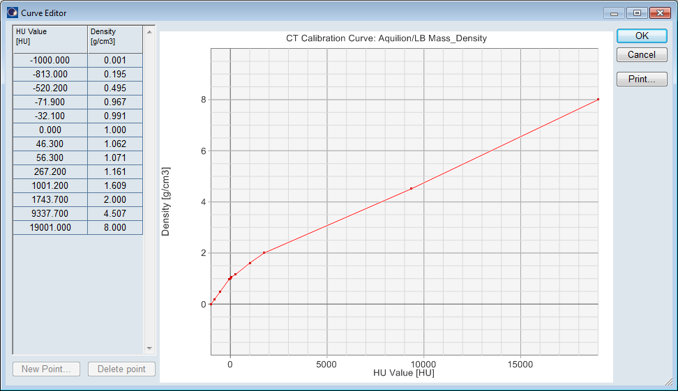
We weighted Head and Body values 1:1 and recalibrated the result to 0 HU for water. This gives the final Mean HU values, which are used for the EDens and MDens calibration curves:
| Material | Inhale | Exhale | Adipose | Breast | Water | Muscle | Liver | B200 | B800 | B1500 | Titan. |
|---|---|---|---|---|---|---|---|---|---|---|---|
| Rel. EDens | 0.190 | 0.489 | 0.952 | 0.976 | 1.000 | 1.043 | 1.052 | 1.117 | 1.512 | 1.859 | 3.735 |
| Rel. MDens | 0.195 | 0.495 | 0.967 | 0.991 | 1.000 | 1.062 | 1.071 | 1.161 | 1.609 | 2.000 | 4.507 |
| HU-Body | -806.7 | -509.0 | -73.3 | -34.8 | -6.5 | 37.7 | 48.3 | 238.9 | 930.9 | 1636.2 | 8702.8 |
| HU-Head | -827.7 | -539.9 | -78.9 | -37.7 | -1.9 | 46.5 | 56.0 | 287.3 | 1063.2 | 1842.9 | 9964.3 |
| Water-Calib | 4.2 | 4.2 | 4.2 | 4.2 | 4.2 | 4.2 | 4.2 | 4.2 | 4.2 | 4.2 | 4.2 |
| Mean HU | -813.0 | -520.2 | -71.9 | -32.1 | 0.0 | 46.3 | 56.3 | 267.2 | 1001.2 | 1743.7 | 9337.7 |
The curves have to be finalized by putting a -1000 HU point for Air at the beginning.
Converting EDens Tolerances into HU Tolerances
According to the recommendations of the SGSMP regarding peripherals, the relative electron density for values up to 1.5 should be within a tolerance of 0.05. For higher electron densities (> 1.5) the tolerance is 0.1.
We model the function EDens(HU) as piecewise linear interpolant in Matlab. With the EDens calibration based on the Mean HU values, the EDens tolerance band can then be converted into a HU tolerance band. The HU tolerance interval is not symmetric, because the slope of the function changes at each data point.
| Material | Inhale | Exhale | Adipose | Breast | Water | Muscle | Liver | B200 | B800 | B1500 | Titan. |
|---|---|---|---|---|---|---|---|---|---|---|---|
| Rel. EDens | 0.190 | 0.489 | 0.952 | 0.976 | 1.000 | 1.043 | 1.052 | 1.117 | 1.512 | 1.859 | 3.735 |
| EDens Tol. | 0.050 | 0.050 | 0.050 | 0.050 | 0.050 | 0.050 | 0.050 | 0.050 | 0.100 | 0.100 | 0.100 |
| Min HU | -862.2 | -569.2 | -120.3 | -97.1 | -73.8 | -9.4 | 2.2 | 105.0 | 815.4 | 1529.7 | 8932.9 |
| Mean HU | -813.0 | -520.2 | -71.9 | -32.1 | 0.0 | 46.3 | 56.3 | 267.2 | 1001.2 | 1743.7 | 9337.7 |
| Max HU | -764.0 | -471.8 | 2.2 | 28.0 | 54.1 | 189.3 | 218.5 | 360.1 | 1215.2 | 2148.5 | 9677.3 |
The B1500 insert for example should give between 1529.7 and 2148.5 HU in any scan. The measured HU-Body value is 1636.2, HU-Head is 1842.9, which means that B1500 is within tolerance (at least regarding the investigated dependence of HU on phantom size).
The Titanium point on the other hand is out of tolerance: HU should be within 8932.9 and 9677.2, but the measured range is 8702.8 (HU-Body) to 9964.3 (HU-Head). Even within the scanned Titanium rod, the range of HU is larger than the width of the tolerance band. This clearly shows the limits of the CT scanner.