|
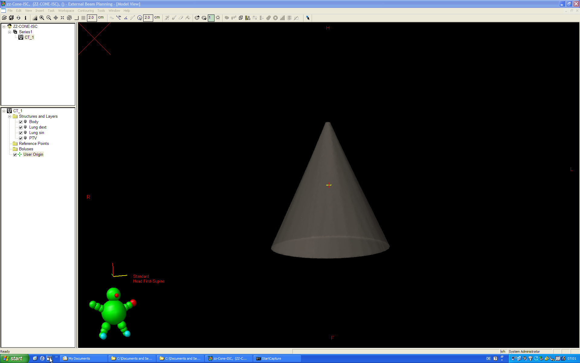
| The treatment planning
process starts by placing the fields as usual. This is the "patient"
I created for this demo: |
|
Fig.1:
"Testpatient" for ISC. |
| |
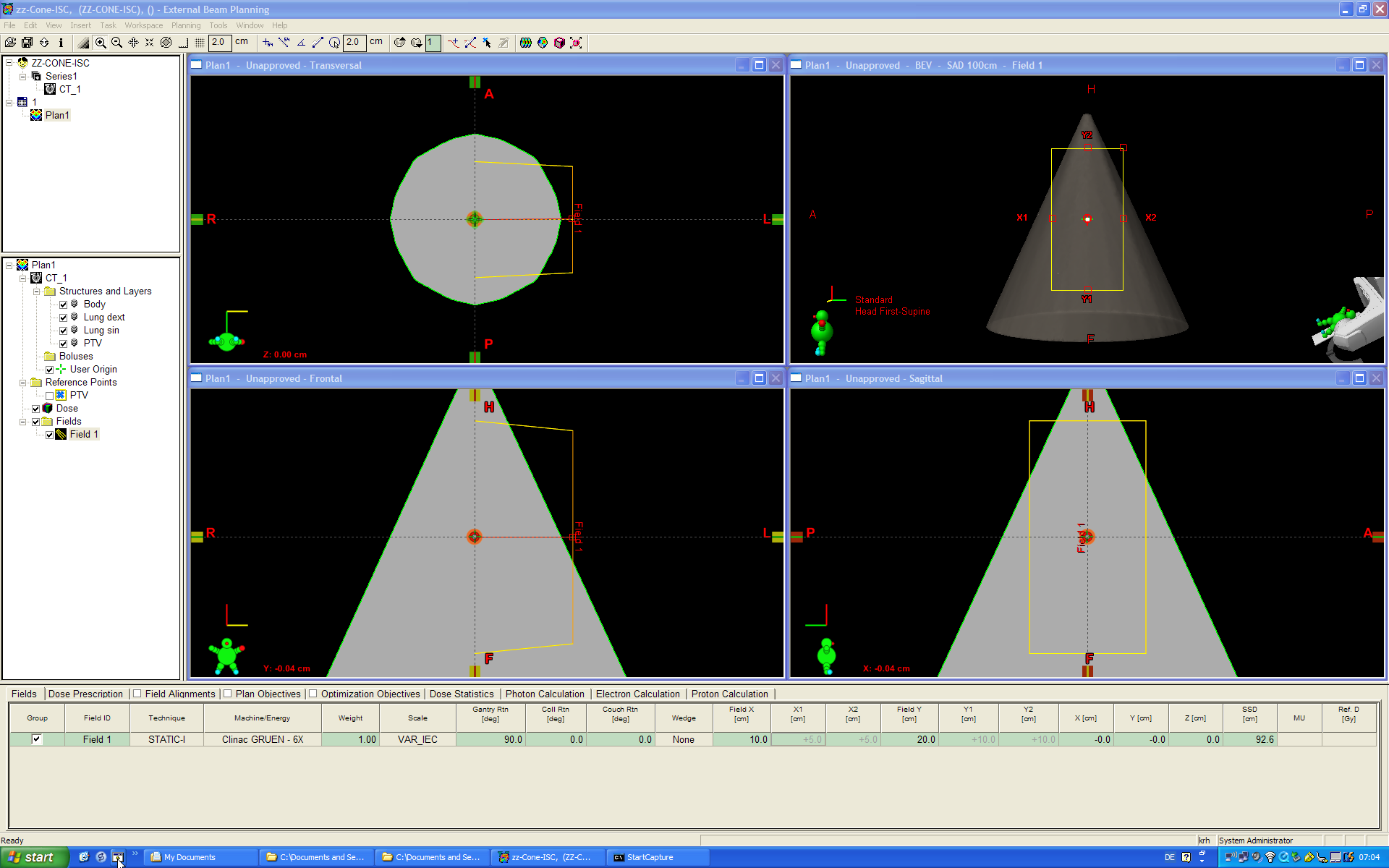
The plan will have
two opposing fields. The first field is created with Gantry 90°. One
can see that the "patient diameter" is very different at different
positions within the field: |
|
Fig.2:
Would be no easy task for a conventional wedge filter. |
| |
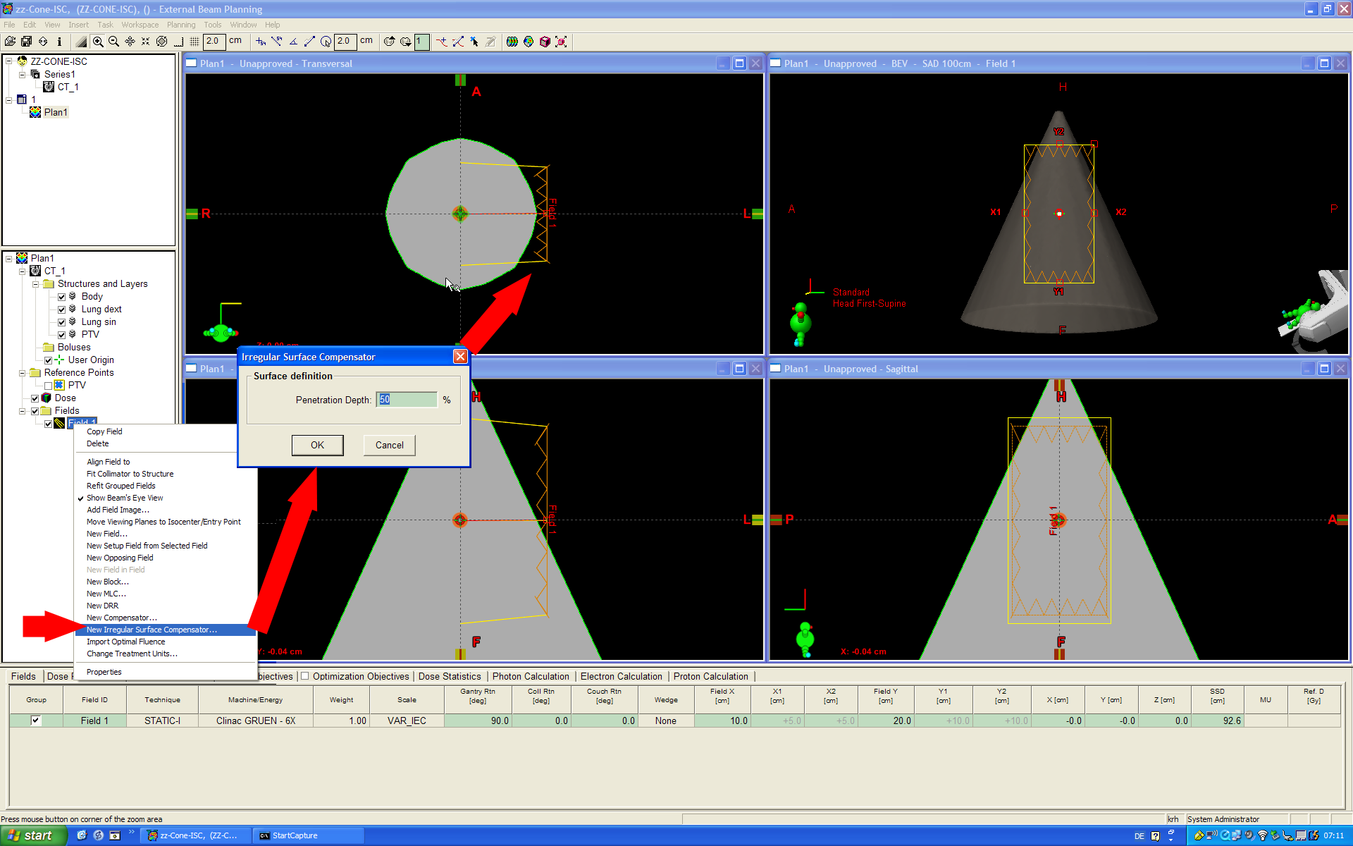
The next step is
to add an ISC as accessory to the field and to specify the penetration
depth. Here, 50% is chosen. The following calculation of the optimal fluence
matrix takes a few seconds. The field now has a characteristic outline: |
|
Fig.3:
The outline of the field indicates the fluence matrix. |
| |
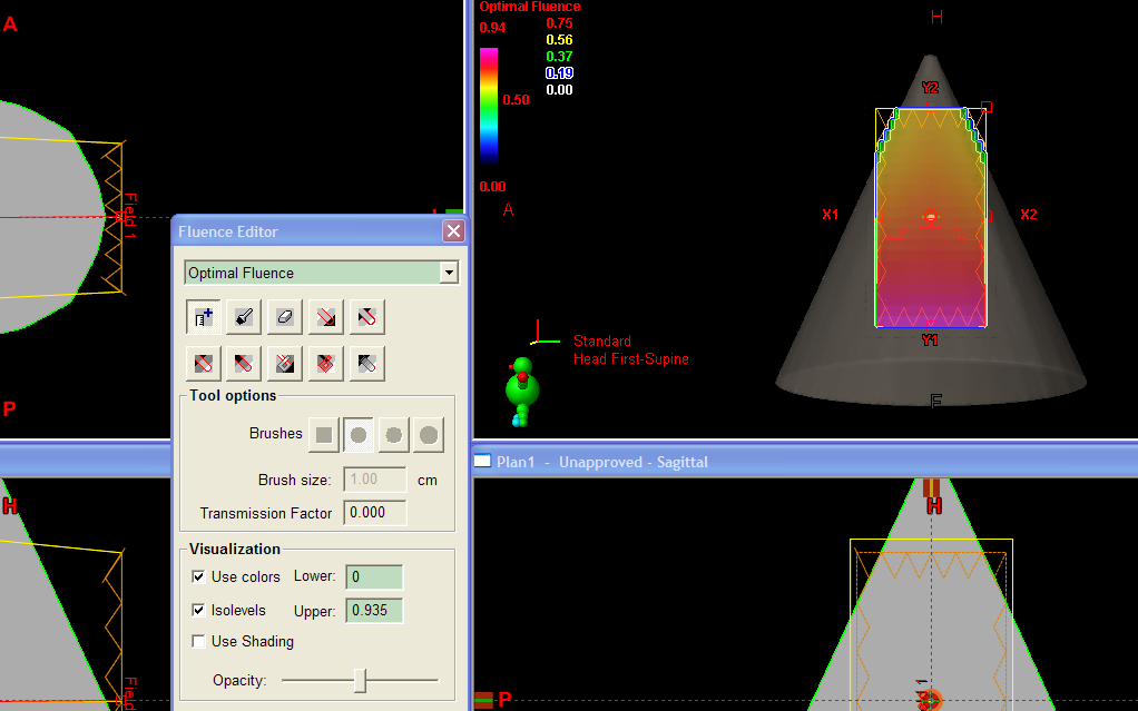
The optimal fluence
matrix can be visualized and changed with painting tools as appropriate. |
|
Fig.4:
The optimal fluence can be visualized or edited in any way, changing the
local intensity of the beam. |
| |
We have not decided
yet how to deliver the fluence matrix. Now we could export the matrix
to a milling machine. Instead, we choose the DMLC: |
|
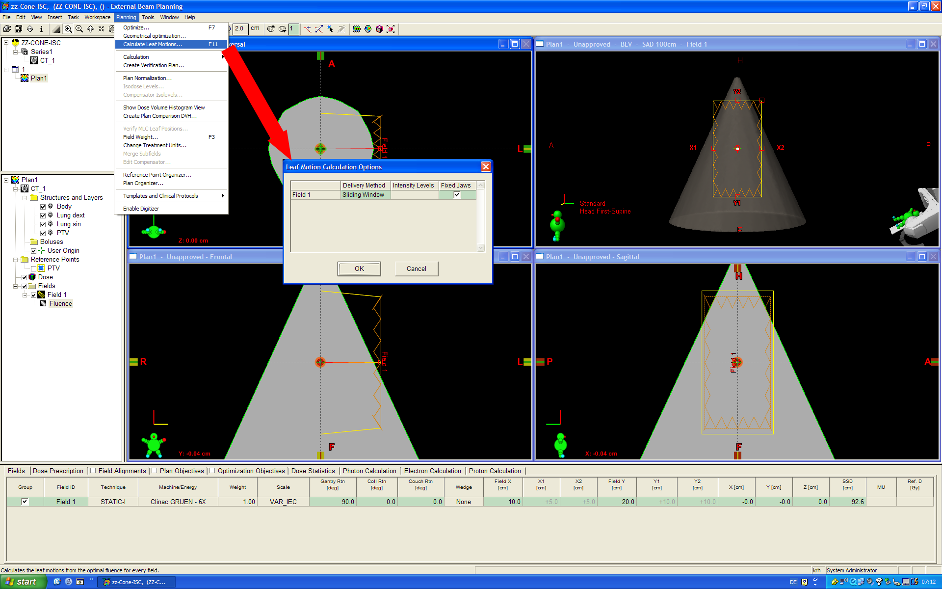
Fig.5:
Choosing Sliding Window will not only generate the deliverable MLC sequence,
but also an "Actual Fluence" matrix, which takes physical properties
of the MLC into account (leaf transmission, etc.). Only this Actual Fluence
will later be used to calculate dose. |
| |
The resulting DMLC
motion can be visualized in Beams-Eye-View. Depending on complexity, the
sequence can have up to 400 segments. |
|
Fig.6:
This field has 77 segments. In reality, the movement is much smoother.
In the animation, only every second MLC segment is shown. On the linac,
true leaf movement is always continuous, even if there are only a few
segments. There are no "jumps", as with step-and-shoot, since
the MLC controller linearly interpolates leaf positions between two neighbouring
segments. |
| |
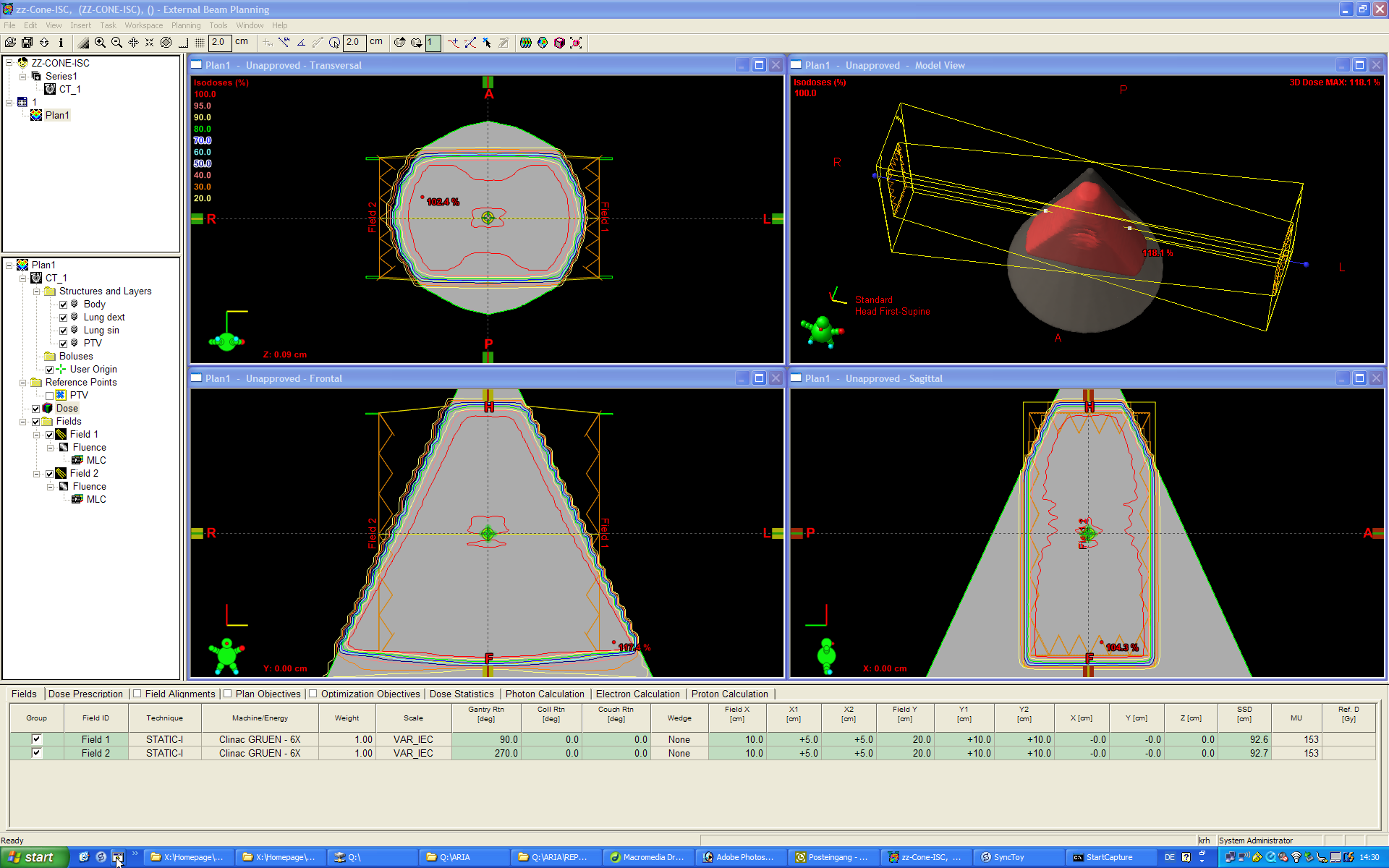
The next step is
to place the opposing field (not shown) and to calculate dose. The result
looks quite homogeneous along the symmetry axis: |
|
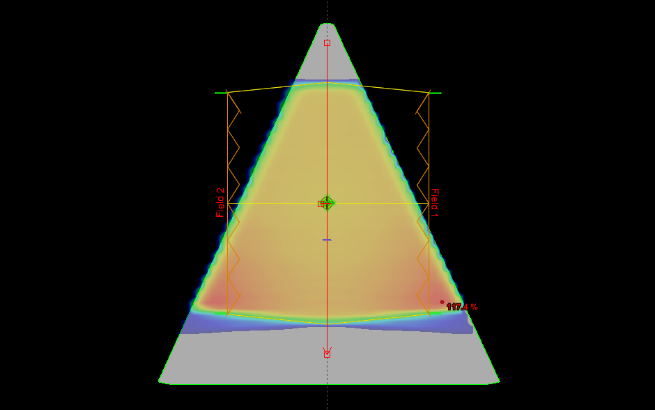
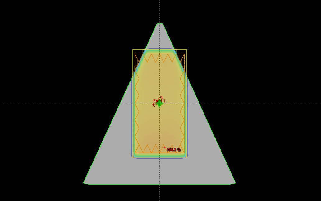
Fig.7:
Dose displayed in color wash. Two opposed fields with Gantry 90° and
270° are seen from top. To reach the goal, fluence has to be increased
in the lower part of the image, which leads to "hot" regions
of 117.4% dose (100% are at isocenter). The red arrow is a longitudinal
dose profile, ... |
| |
|
Fig.8
... which reveals that dose slightly increases to the caudal edge of the
field (where the "patient" has the biggest diameter). But all
in all, dose is quite homogeneous. |
| |
|