I use Mathematica for two things: first, without the use of the LFC, it is easy to read in DynaLog data directly and plot trajectories etc., as shown in the basics page. But trajectories can only show a single leaf pair. I prefer to calculate 2D images that show all leaves simultaneously. In these plots, the vertical axis always shows the leaf number, the horizontal axis the DynaLog record number:
|
|
The plot contains (TA-PA), that means true minus planned leaf positions for leaves of carriage A (leaves A1-A10 are shown). Values are from Dynalog. The odd leaf numbers go first. When they stop, the even leaves start.
In the next example one can see that it makes not much difference if one plots the leaf position error,
or the velocity,
if one looks for leaves that go too slow. Here leaf 7A is slower than the rest, which leads to a higher leaf position error. Both plots identify leaf 7A. The leaf motion pattern is the same as the example shown in the basics page.
The second category of Mathematica usage involves fluences precalculated with the LFC. Computing them directly in Mathematica is also possible, but my notebooks evaluated too slowly, because I used a procedural programming approach (and nested loops are not the domain of Mathematica). Another thing is that when Mathematica notebooks get too large and complex, they possibly contain errors. And the resulting error messages sometimes do not help a lot:
So life became easier when fluences were calculated in LFC, and Mathematica was only used for plotting.
Here is a 3D view of a true fluence. Leaves move from left to right, as shown in the movie. All leaf pairs are closed according to plan. The hold-offs that appeared in the right part lead to the "ripples in the sea of fluence":
 |
 |
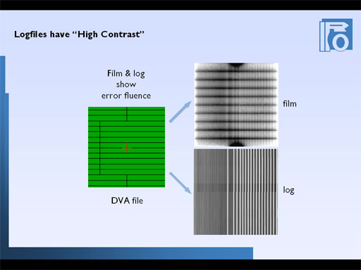
Again, when comparing log to film, one can see the agreement. One can also see the inherent high "contrast" of the logs.
Zooming in the 3D view, one can explore the details. Here, about 5mm of leaf pair 16 (the first that is moving) are shown:
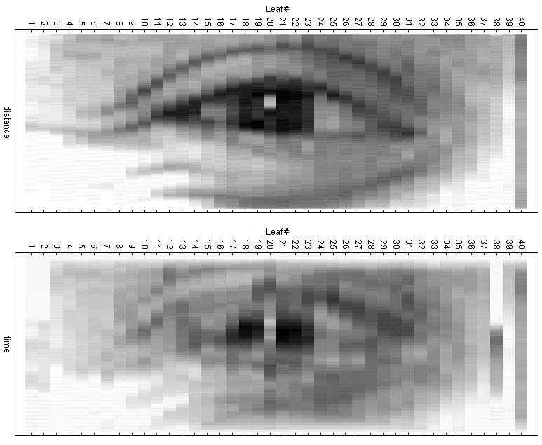
For those of you who have already looked at the eye-quiz, the following example will look familiar. The upper image shows the "true fluence", calculated from the DynaLog files. The image below shows the leaf gap of each leaf as a function ot time, gap width encoded in grayscale. Darker pixels mean wider gap. Another way of looking at things.
back to DMLC home