Portal Dosimetry in ARIA10
History
For many years, there was no update of the Varian Portal Dosimetry (VPD) tool. Physics was working fine, however, the Analysis Workspace was not very user friendly. It did not offer QA Reports (we printed screenshots instead). It was the beginning of the OBI hype when VPD development came to a halt. At that time, probably all Varian developers had to focus on OBI software.
In 2011, ARIA10 surprised us with a complete redesign of the Analysis Workspace. PD configuration steps and physics are still the same, so the information found here is still valid. But the clinical workflow is now even faster (a complete plan evaluation of several fields is a matter of seconds) and offers more possibilities.
Example Plan
A 5-field treatment plan with 15 MV and Gantry angles 40°, 90°, 180°, 270°, 325° is measured with Portal Dosimetry.
In Eclipse, the portal dose image prediction is calculated with the PDIP10028 algorithm. Since our Clinacs have the old R-Arm, all measurements are performed at Gantry 0°. MLC is Standard80, the aS500 IDU20 detector is set at SDD 105 cm. Dose rate is 300 MU/min.
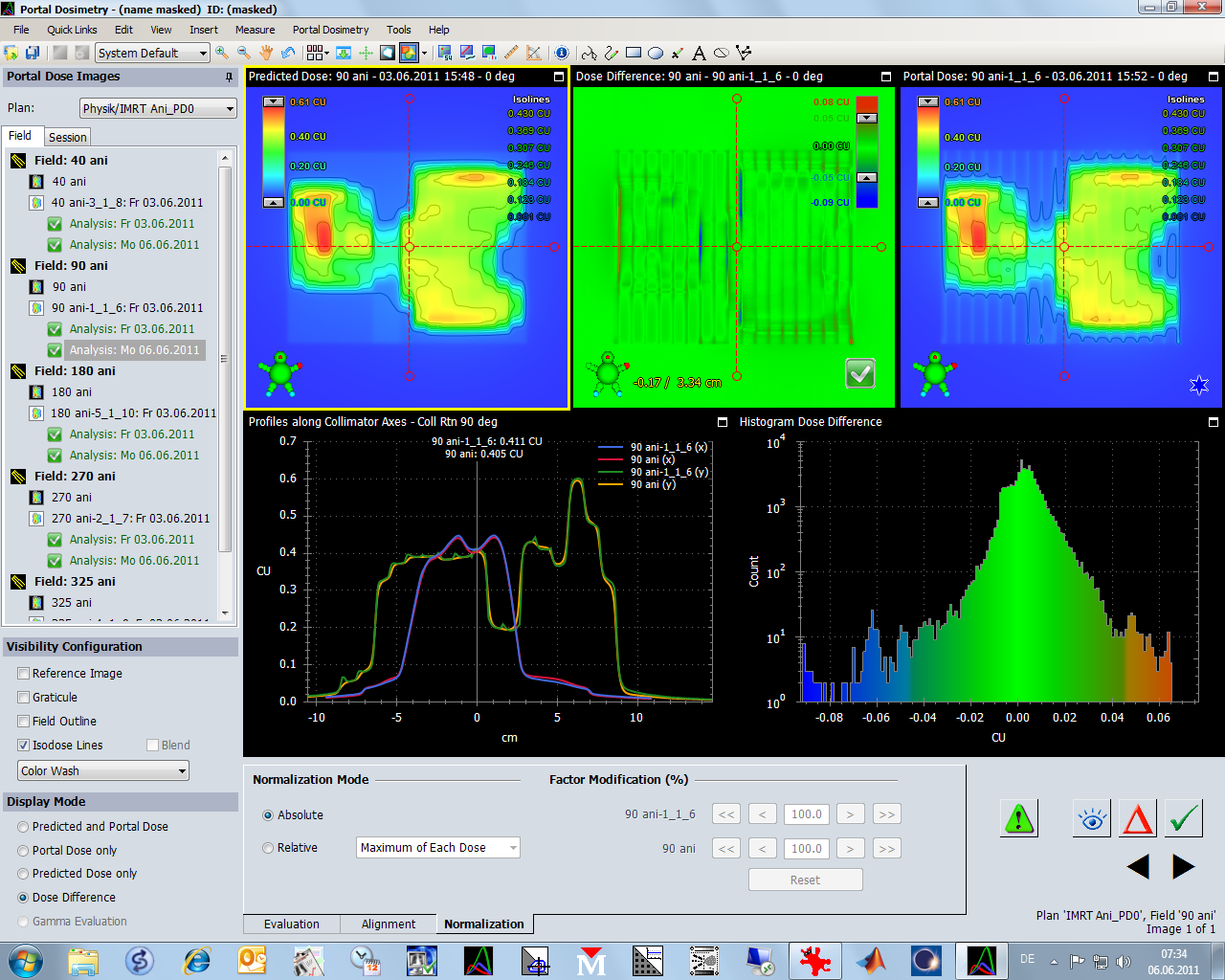
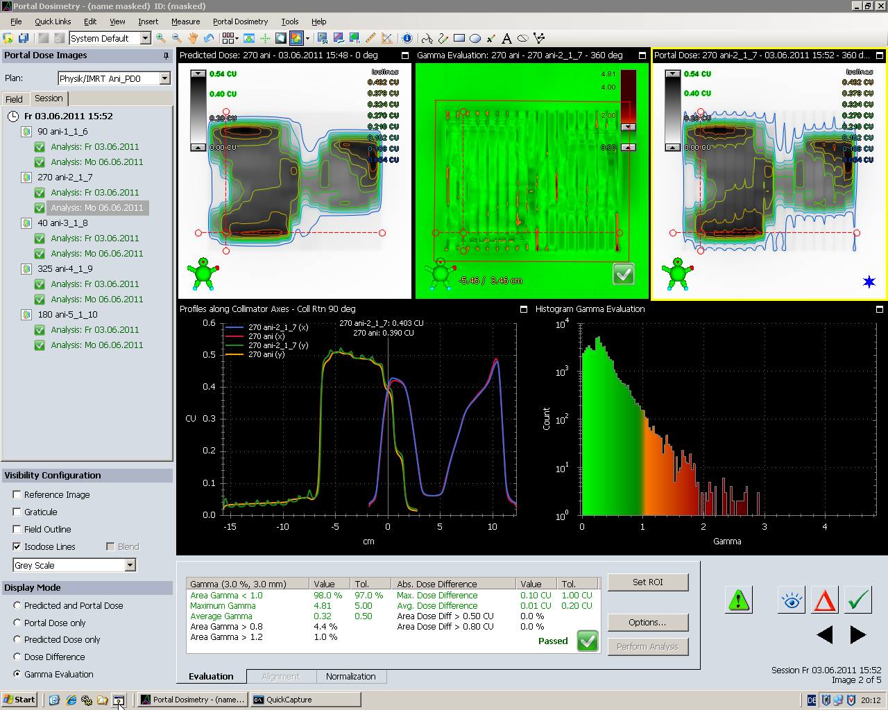
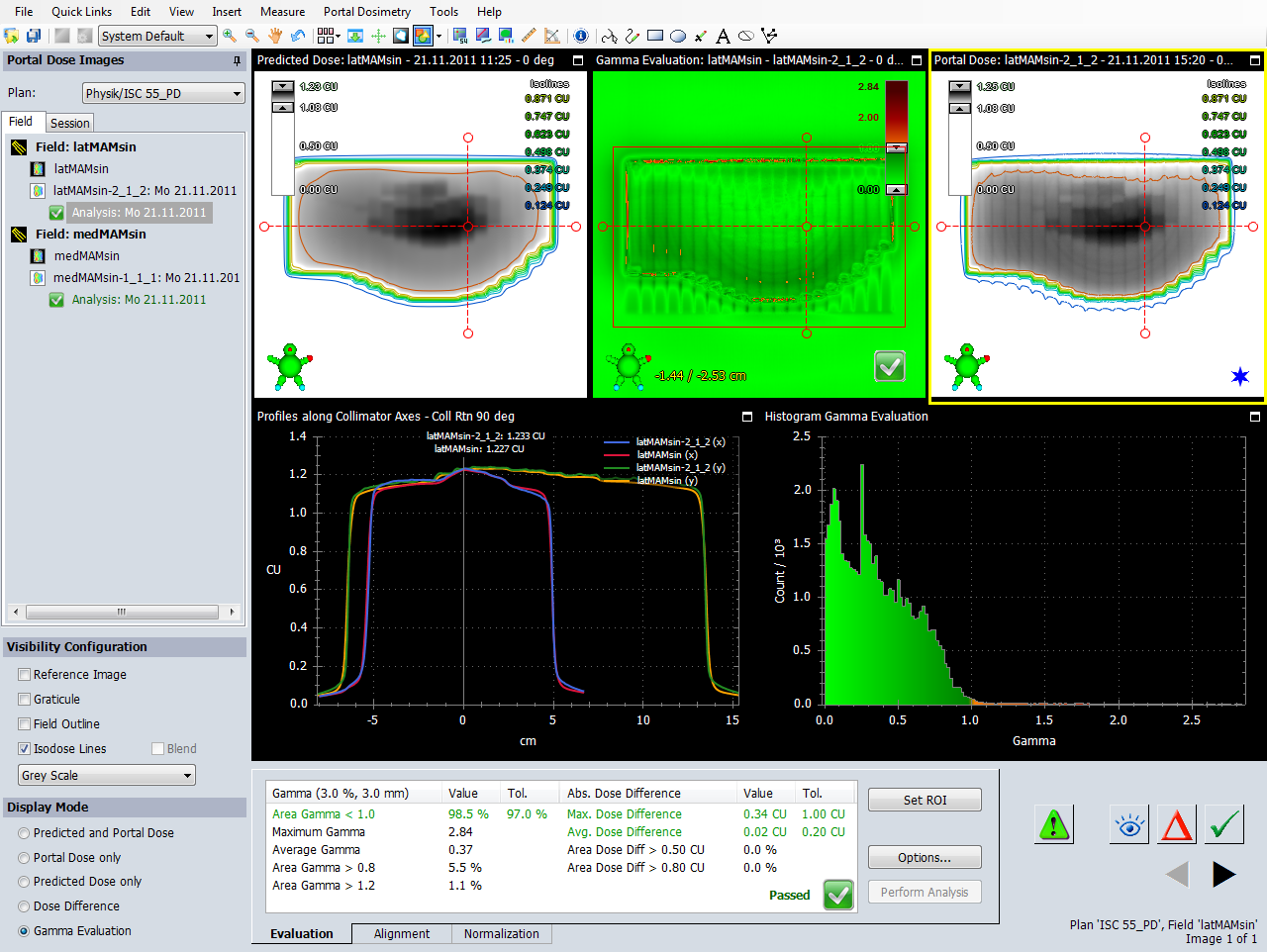
One of the different screen layouts shows predicted and measured dose left and right and the gamma evaluation map in the center of the upper row:
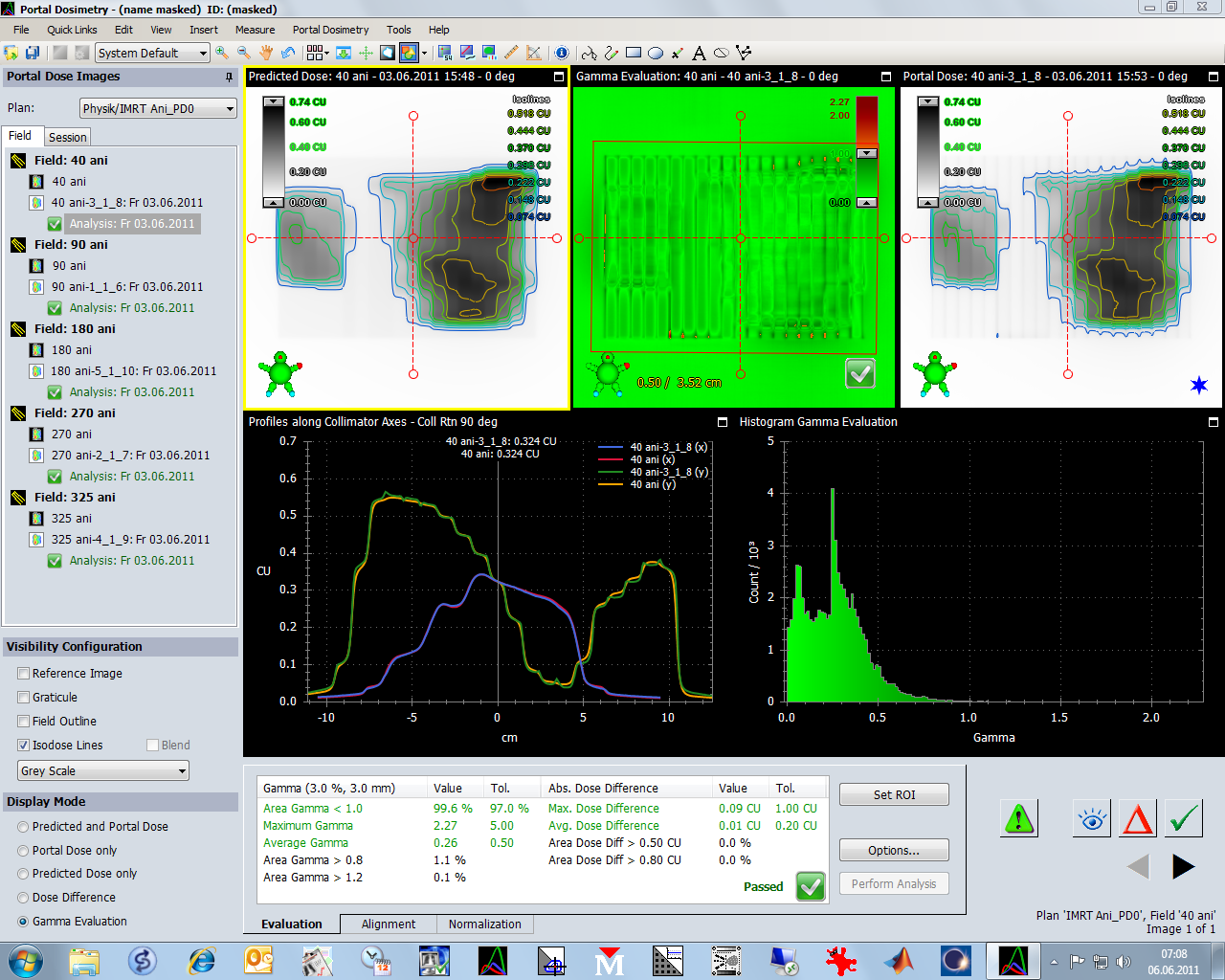
The profile axes can be dragged around with the mouse if they are grabbed at one of the 5 circles. The vertical scale in the profile plot (lower left graph) adapts automatically:
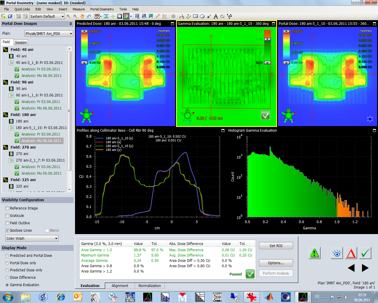
The gamma histogram is in the right half of the second row (here shown in linear scale):
The Evaluation tab in the bottom row sums up the analysis results. Here, 98% of the pixels have a gamma smaller than 1, which is within tolerance (97%). If there is no value in the tolerance column (like for "Area Gamma"), this means that this parameter is not tested in the selected template:
Note: if one of the tests fails, the overall result will be "Failed".
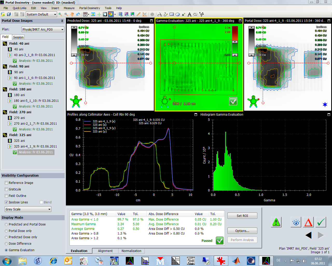
In the left column, for each field an "Analysis" icon is displayed together with the date of the analysis.
You don't have to delete an analysis in order to create a new one! In the next screenshot, a second analysis is created by applying a template (could be a different one) to the plan:
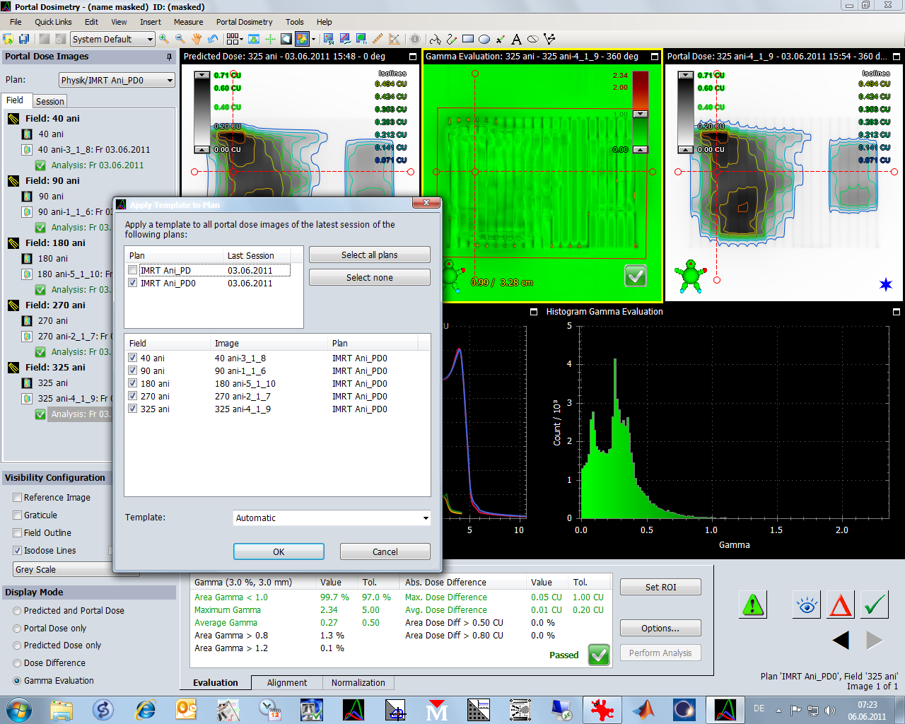
Now each field holds two analyses.
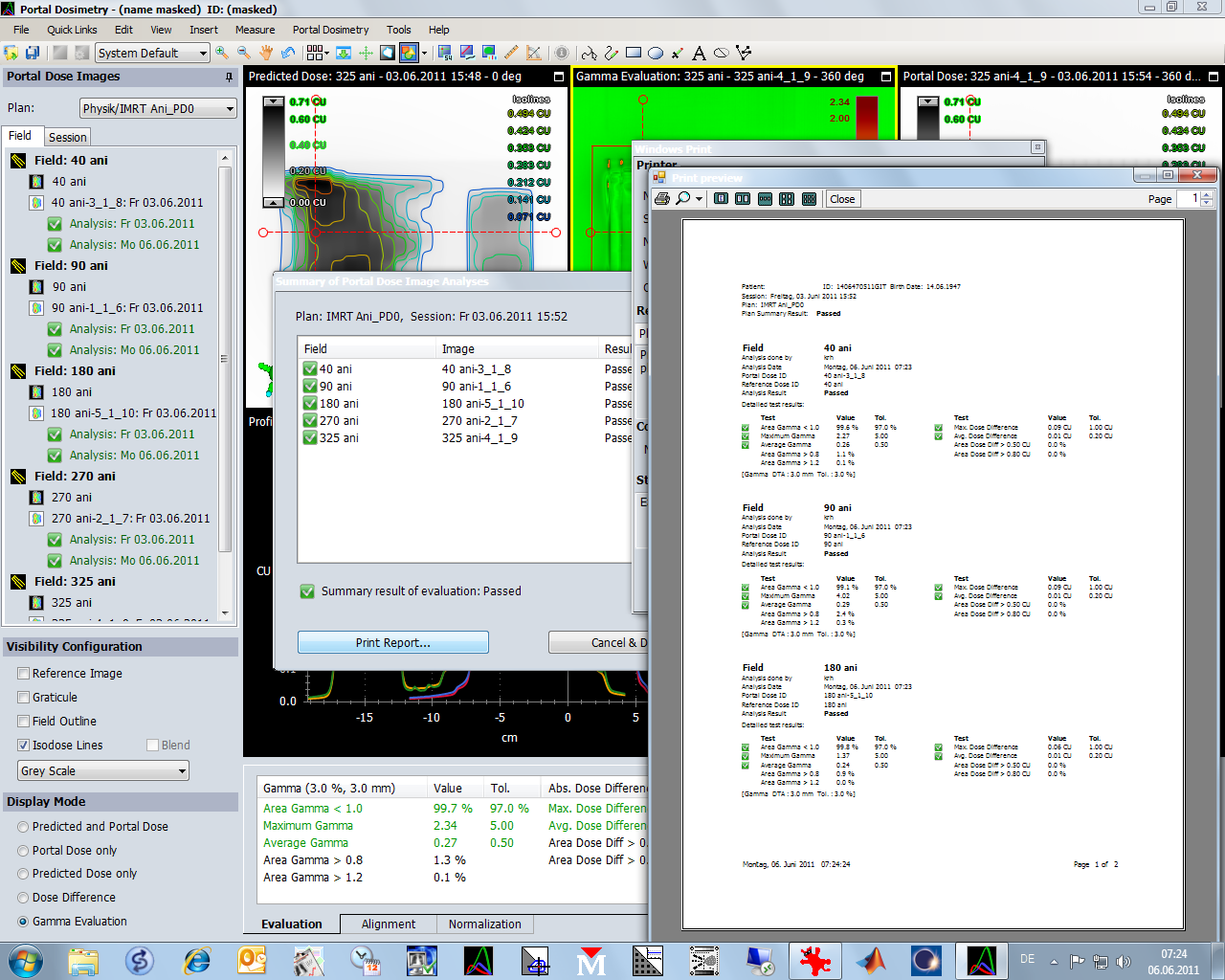
The software automatically runs through the fields, performs image alignment automatically (very convenient with our R-Arm), and displays the overall result:

When "Print Report" is selected, a (configurable) report is generated. This is what we routinely print, sign and archive:
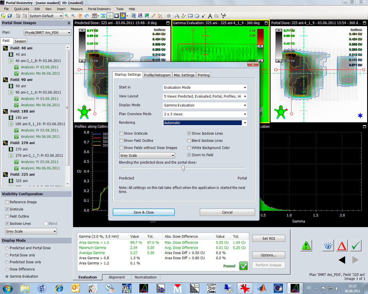
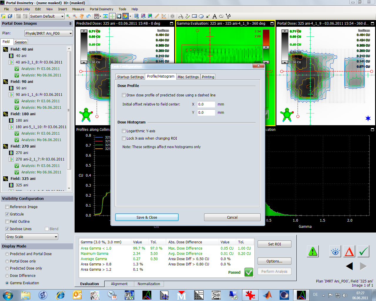
Here are some settings from Task Configuration:

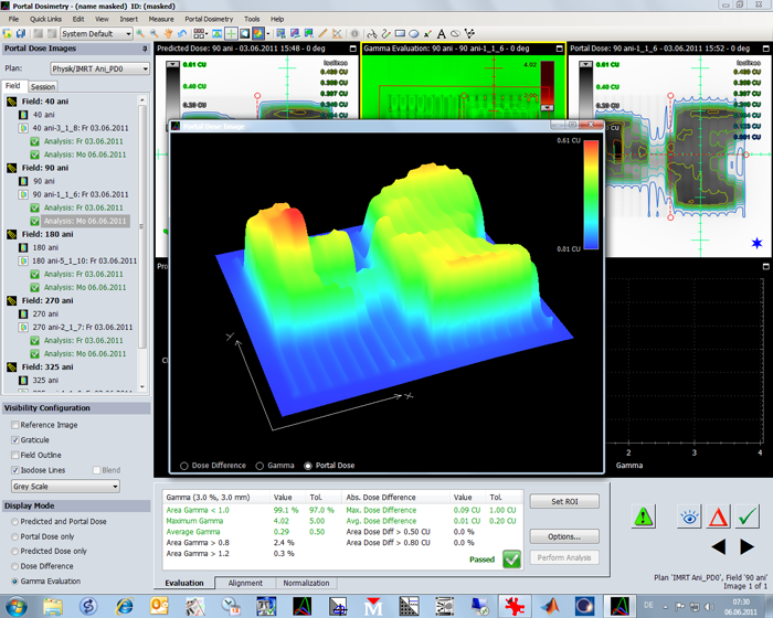
Every software needs some 3D graphs, although they don't give any new information:
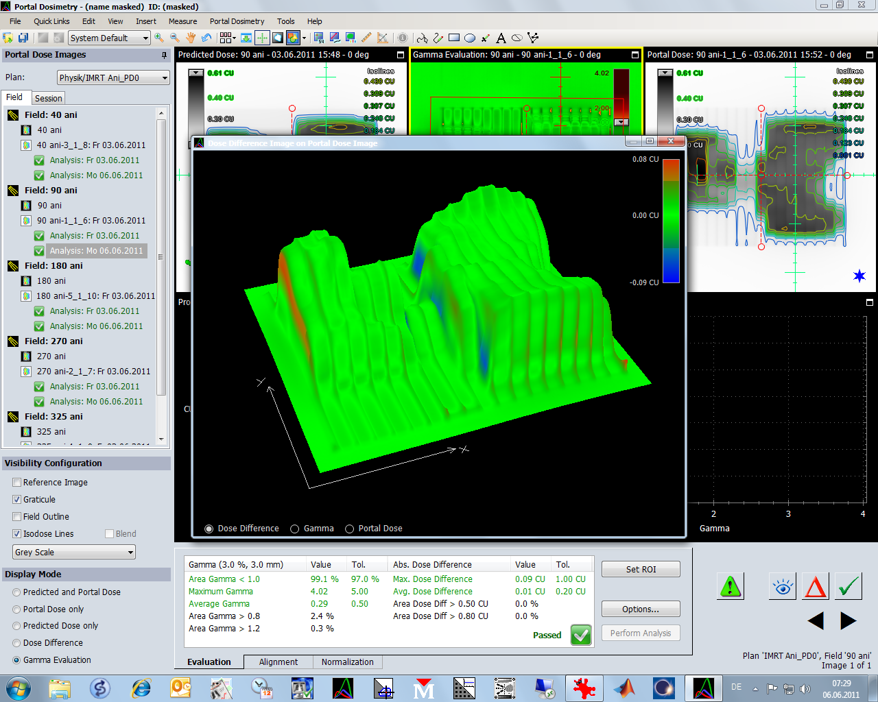
Dose diff, Gamma and portal dose can be visualized in 3D and rotated around with the mouse. (honestly: who needs this?)
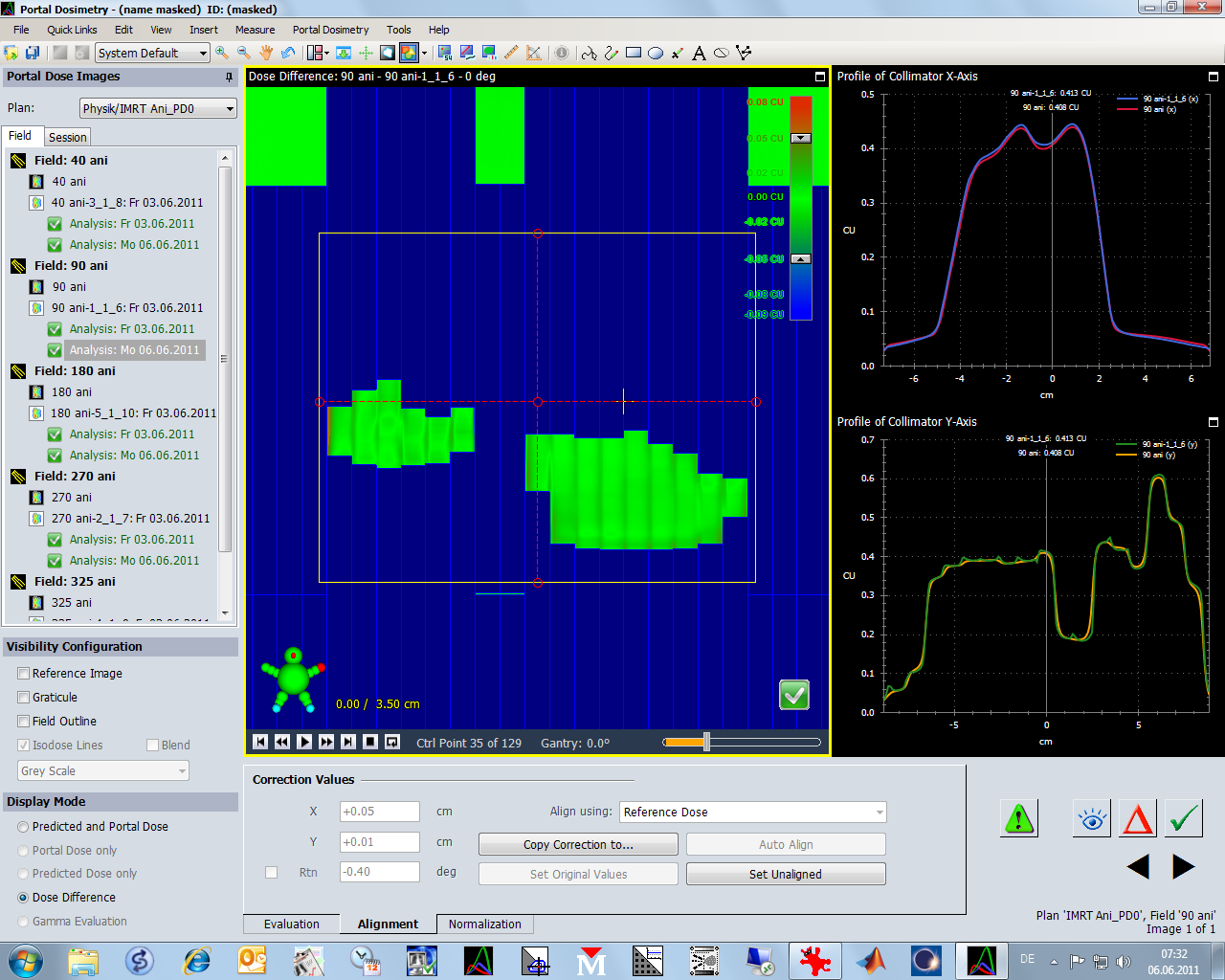
The Dynamic MLC visualization is a more useful tool:
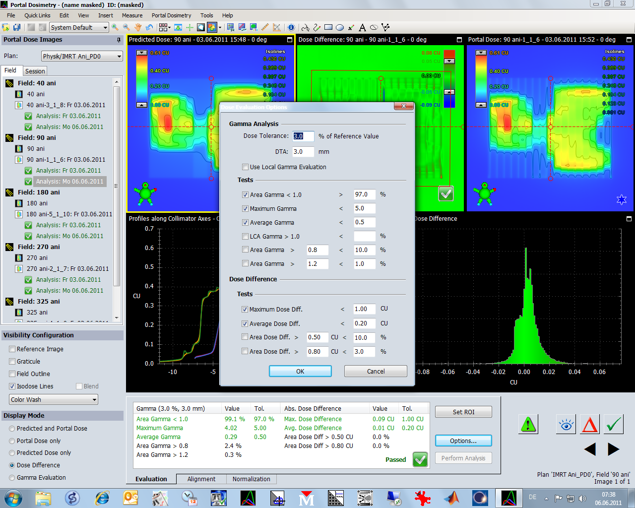
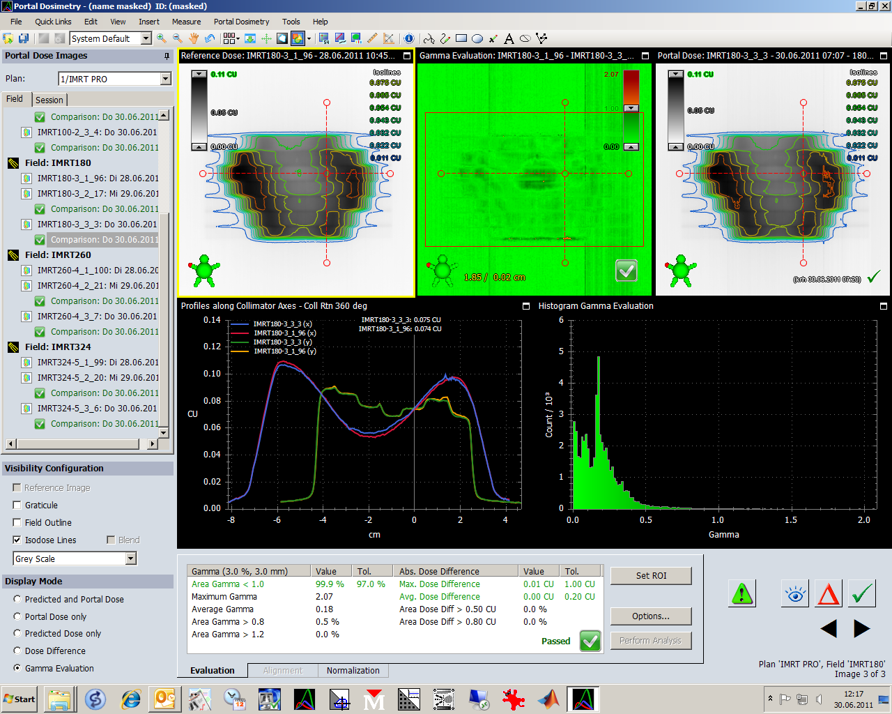
In the next screen, the dose difference is plotted, not the Gamma map. The histogram is in logarithmic scale:
Log scaling visually "blows up" low counts. In this Gamma histogram, only a few pixels have Gamma > 1:
These are the tests we typically use (Maximum Gamma is still tested here, but we stopped this in the meantime):
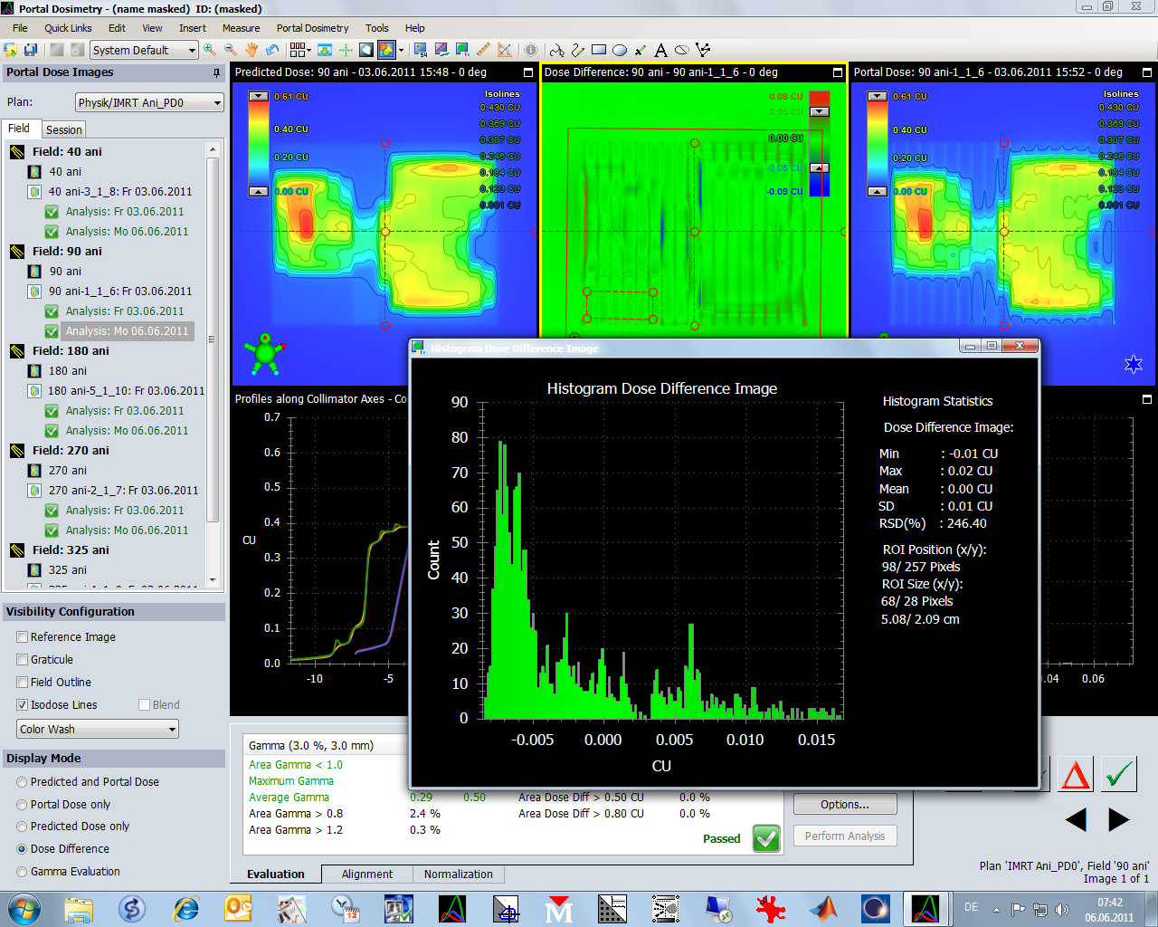
Arbitrary histograms can be generated, here in the small rectangular low dose region of the Dose Difference plot:
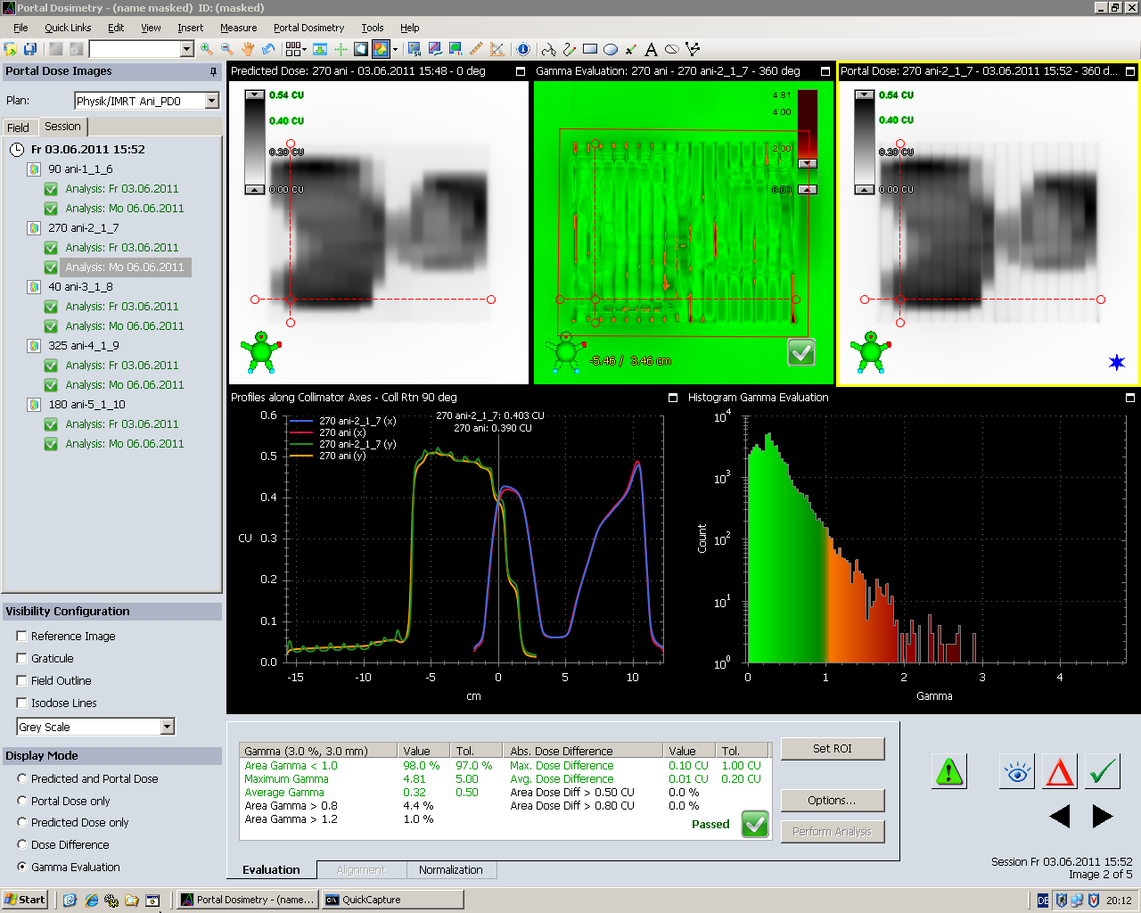
One last remark: is is really useful to plot isodoses over the greyscale Eclipse and EPID images?
After switching off the isodoses, small features in the images (tongue and groove effect in the EPID image) appear:
Review of Daily Patient Images
An interesting feature of the VPD tool is the possibility to compare the transmission images of the daily patient treatments. Here a prostate example:

Instead of comparing prediction and measurement, two measured fluence images are compared. For instance, the images measured during the first and the second fraction. The comparison is invoked by right-mouse-clicking on a measured image:
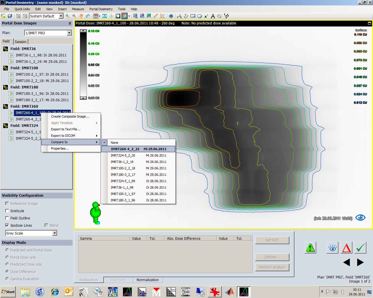
Target images where a comparison makes sense (same Gantry angle) are highlighted in bold. For R-Arm users, the first step should be to click "Auto Align" to align the two images.
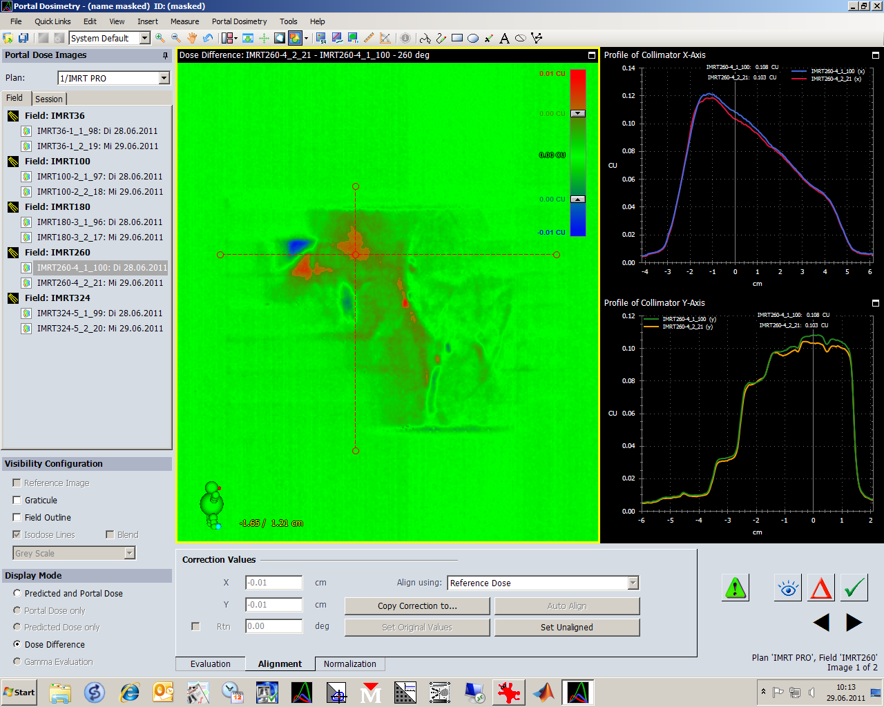
After alignment (Auto Align button gets greyed out), one can use all the typical analysis tools like Gamma Analysis tests, histograms etc. that are known from the pretreatment verifications. This can be used to highlight an air filled rectum that was not there yesterday, etc.
All Evaluations performed are saved to the source image (the one which was right-clicked). It can also hold several evaluations at once:
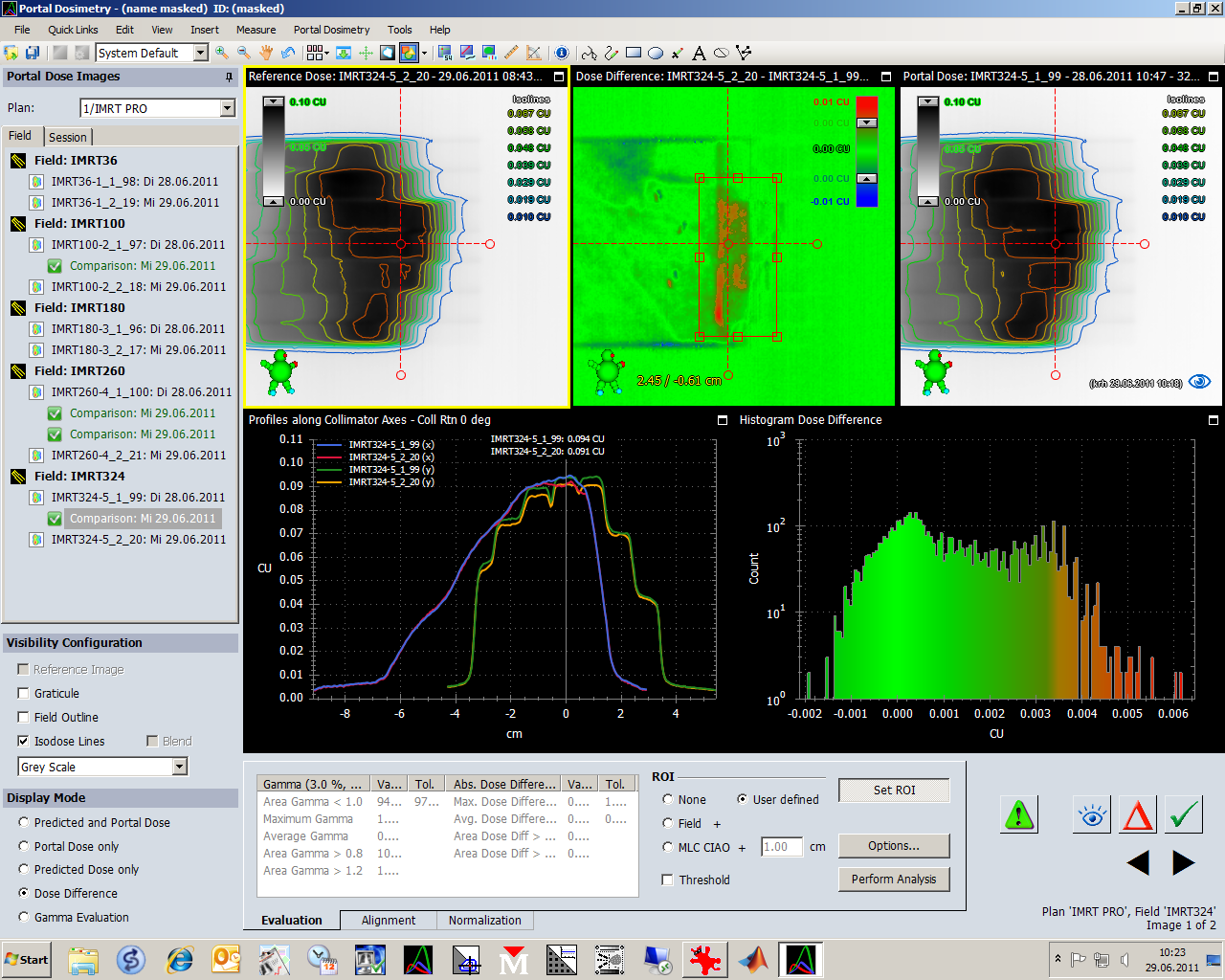
However, interpretations of such difference images are not easy. The source of a measured difference is not always inside the patient. Here, the patient was positioned on the couch a bit more laterally than during the first session. The carbon rail is in the field. As can be seen from the Gantry angle (324°), it is on the exit side:
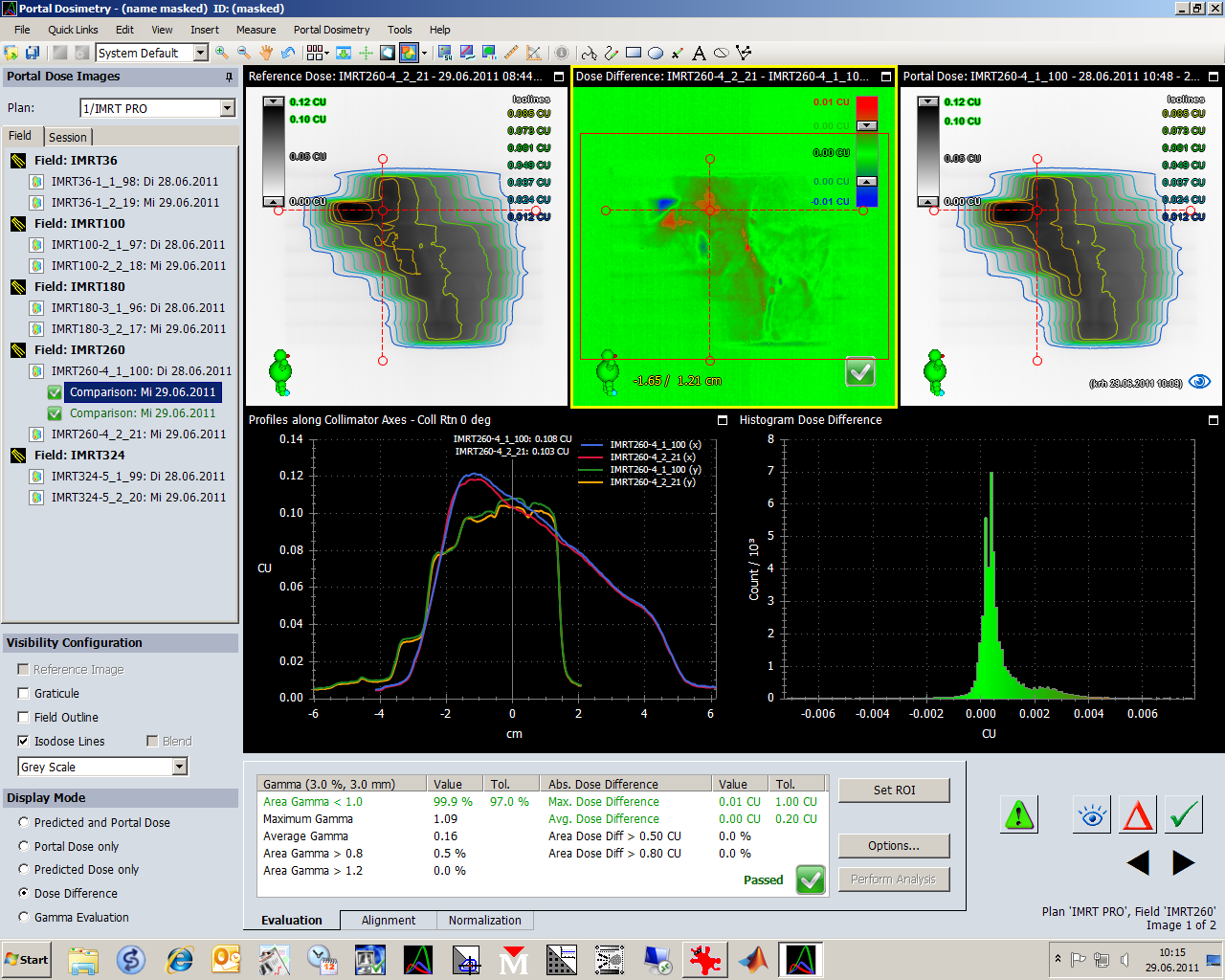
One not regarding the sign of differences. If image "S2 is compared to S1" (right-click on image S2), the matrix S1-S2 is computed, and the result is attached to image S2. This way, if the first session image is taken as reference, daily images can be evaluated, like S1-S2, S1-S3 etc.:
The sign is not intuitive: if the most recent image "x" when compared to the reference image "1"a positive dose deviation is detected in , this means that the most recent image has a LOWER dose than the reference, since S1-Sx is computed and positive.
Portal Dosimetry also works well for ISC (Irregular Surface Compensation), at least most of the time:
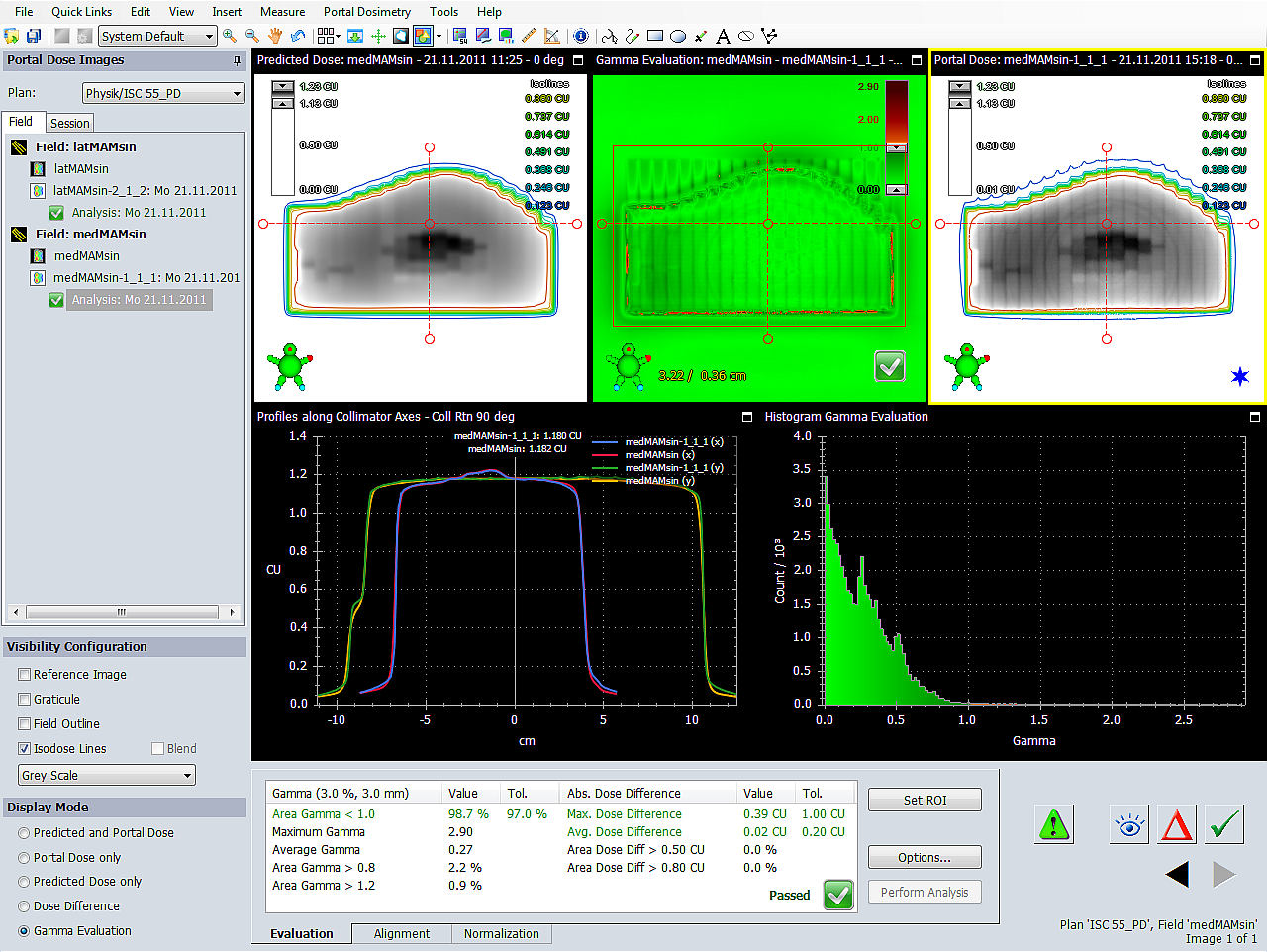
For ISC fields, where large detector areas are irradiated with a significant fraction of MU, we sometimes observe poor agreement in the central detector area. If such a field is remeasured with the 2D-Array, there are no relevant deviations. This indicates that the source of the problem is the aS500 detector, not the field. According to Varian, increased backscatter of the R-arm is the reason for these problems.
Conclusion
Regarding the user interface (graphics, templates, printing etc.), Varian did a good job with the Portal Dosimetry tool in ARIA10. Evaluation is fast and easy. If the patient is already opened on some ARIA workstation in the control room, all you have to say after the end of treatment is "Reload All" > "Edit" > "Apply Template" > "Print Report". This takes a few seconds.
If only the Physics were better ...