AcurosXB is a relatively new Eclipse dose calculation algorithm which solves the coupled linear Boltzmann transport equation (LBTE) for photons and electrons on a grid (see sidebar and Literature).
Materials and Methods
Since the main difference between Acuros and established algorithms like AAA are expected to show up in the presence of inhomogeneities, we focused on this aspect (which is only part of the full commissioning process) and compared calculated and measured planar dose distributions for a restricted subset of setups.
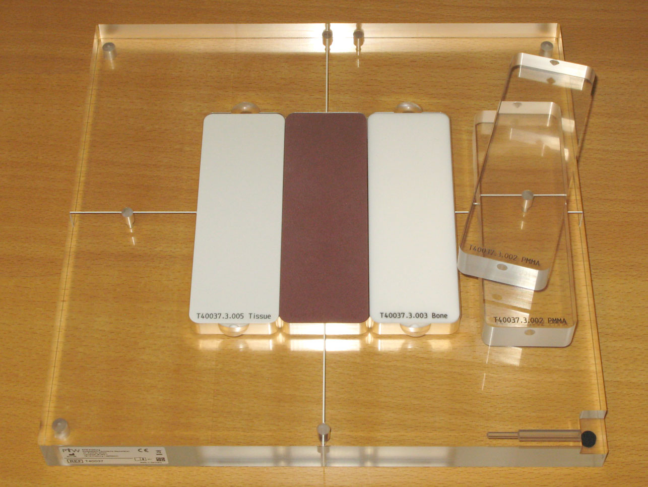
We used the relatively inexpensive PTW IMRT inhomogeneity phantom T40037 (see sidebar). For our tests, we placed the T40037 on top of the 2D-Array OCTAVIUS Detector 729, which has the same outer dimensions of 300x300 mm as the phantom.
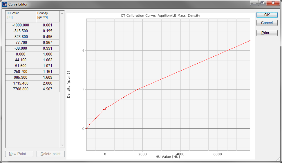
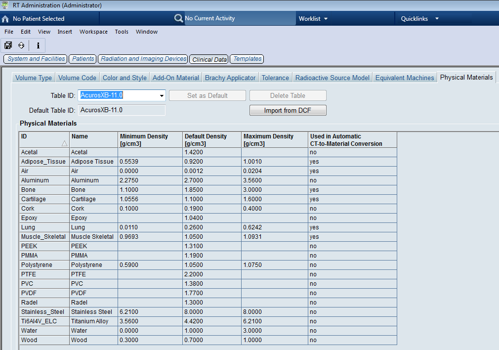
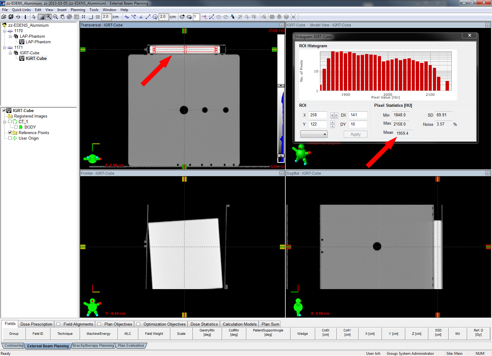
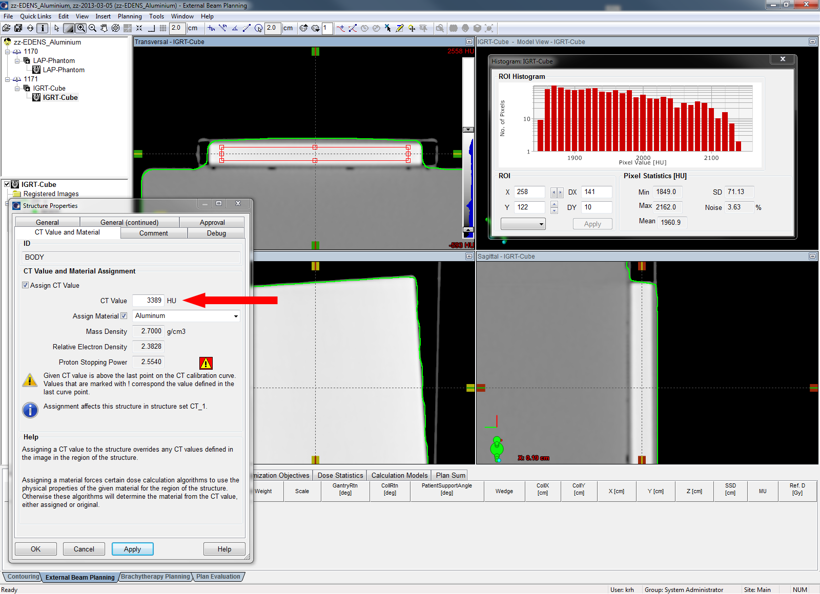
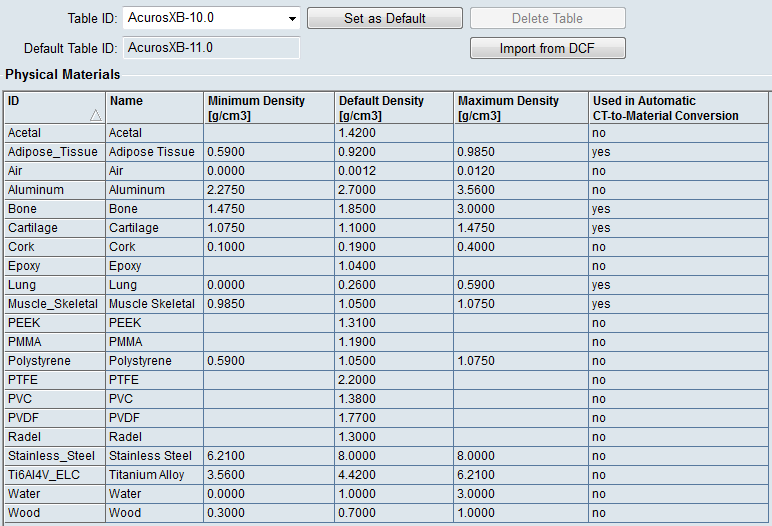
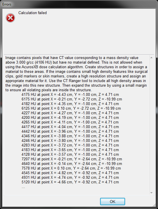
The whole setup was CT scanned on the ToshibaLB scanner using standard clinical protocols (120 kV, TCOT, slice spacing 1 mm), then imported in Eclipse and contoured. Since AcurosXB version 10 works with mass densities and does not perform an automatic material assignment if voxels have HU numbers beyond a certain limit (this is somewhat improved in AcurosXB version 11), we created a "hidens" dummy structure and assigned the material PTFE (2.2 g/cm3) to it. It doesn't really matter which material is chosen, because the voxels Acuros complains about are never in the region of dose calculation, but are almost always screws and cables at the edges of the phantom. However, in clinical cases (teeth), the material asignment becomes important.
Workflow with the inhomogeneity phantom T40037
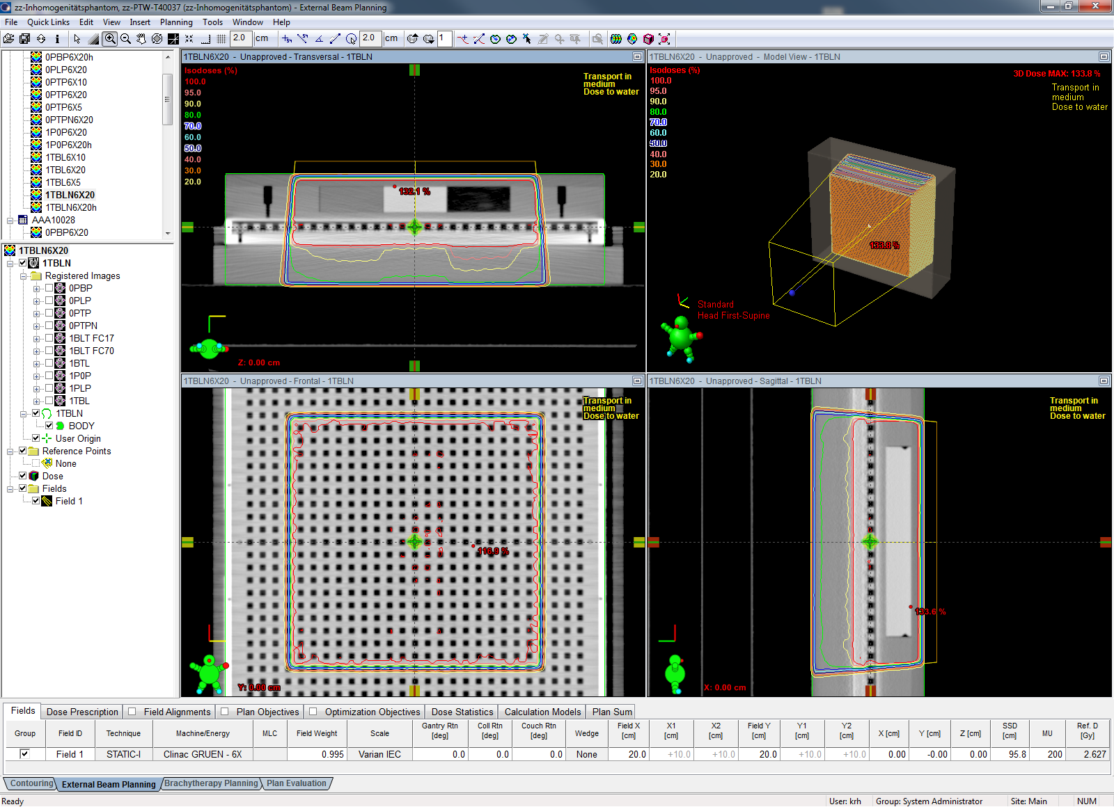
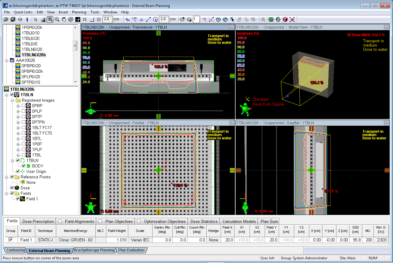
The whole setup (phantom plus 2D-Array) was scanned several times with different arrangements of the inhomogeneity blocks Bone (B), Tissue (T), PMMA (P), Lung (L) and Air (0) and two different buildups: either with one cm of RW3 on top of the T40037 (1) or without any extra buildup (0). The thickness of the inhomogeneity blocks is 20 mm. The base plate made of PMMA adds another 5 mm of PMMA between the inhomogeneity inserts and the surface of the 2D-Array. Since three inserts can be placed inside the phantom in different ways, we used a certain naming convention. A setup of 1TBL for instance means: 1 cm RW3 as buildup, with the inserts Tissue, Lung, Bone from left to right:
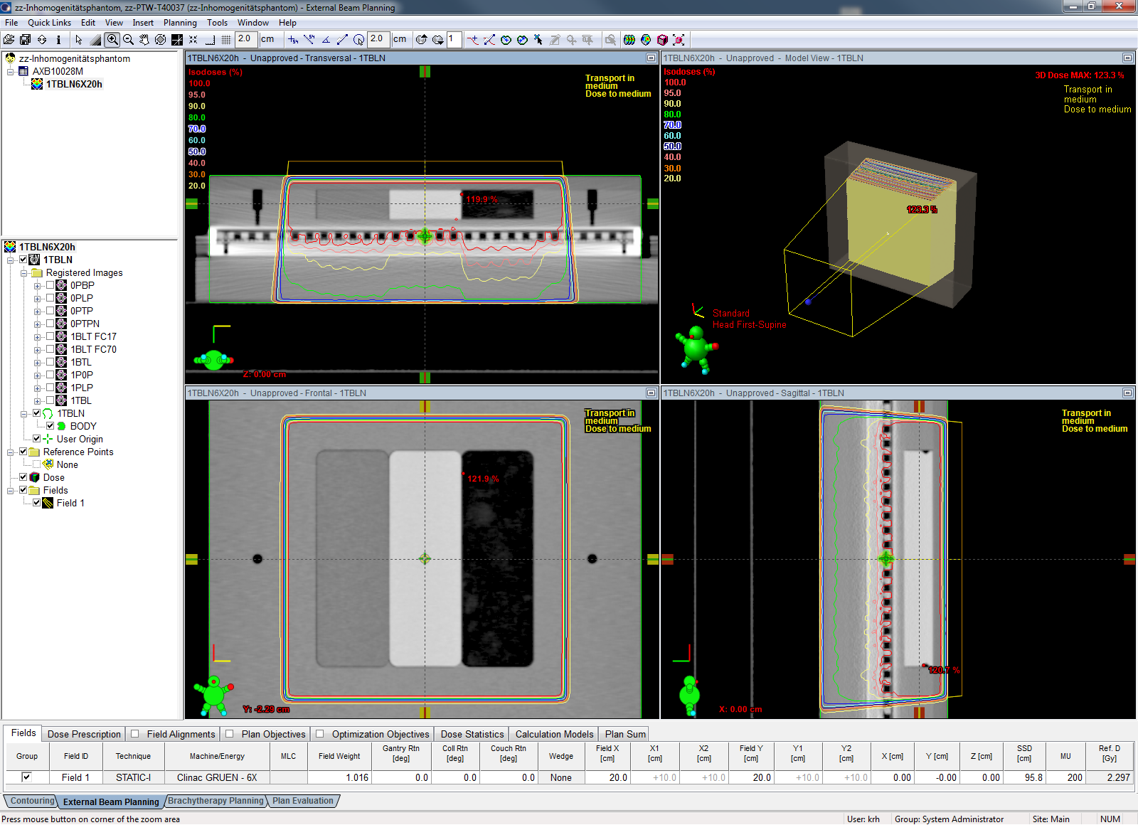
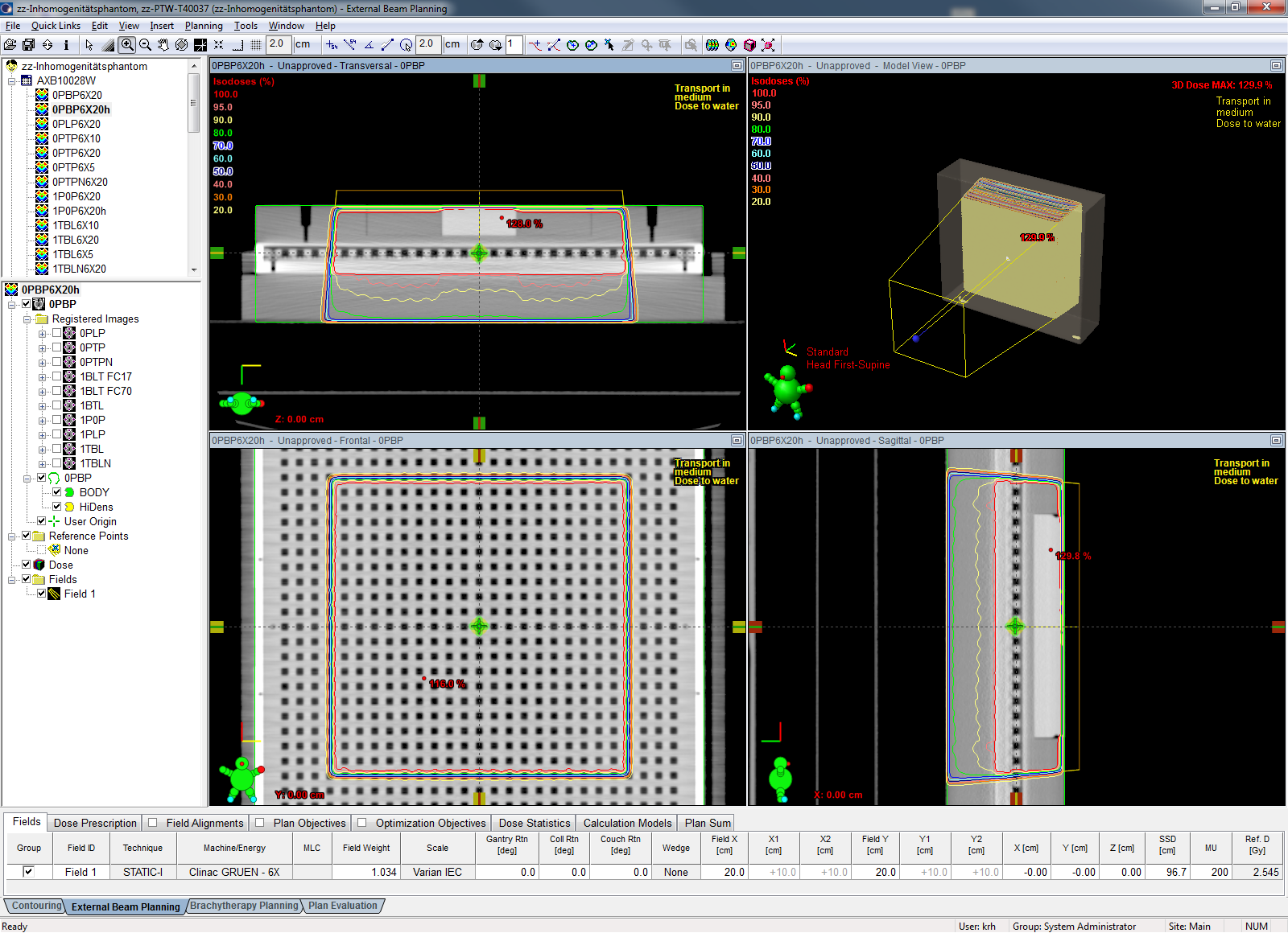
(Calculation with AcurosXB for the setup 1TBL, reporting dose to medium)
All plans were calculated with a 6 MV flattened beam, 20x20 cm field size and calculation grid sizes of 1.5 mm and 2.5 mm for a fixed 200 MU. The algorithms used were AAA version 10.0.28 and AcurosXB (AXB) version 10.0.28. The AXB calculations were performed both with "Transport in medium, Dose to medium" (D2M), and "Transport in medium, Dose to water" (D2W). This means that for a certain calculation grid size, a single measurement was compared to three different calculations.
The beams were measured on our Clinac 2300C/D. The agreement between the dose matrix calculated in the effective measurement plane of the OCTAVIUS Detector and the measurement was evaluated using VeriSoft 4.2 software. The Gamma method was used with a criterion of either 2%/2mm or 3%/3mm (see tables). The result was the passing rate, given in percent of the number of evaluated points (which were always 729, i.e., the whole 2D-Array). The passing rate is equivalent to the so-called Gamma Agreement Index (GAI). A GAI of 100% means that all evaluated points pass the Gamma criterion.
The evaluations are relative in the sense that a homogeneous buildup was chosen as a "reference field". The measured reference field was used to establish a kUser factor, by averaging measured dose over the central 9x9 chambers. This overall factor was successively applied to all measured inhomogeneous fields. By normalizing to the reference field, it is "postulated" that Eclipse correctly calculates the reference field.
Results
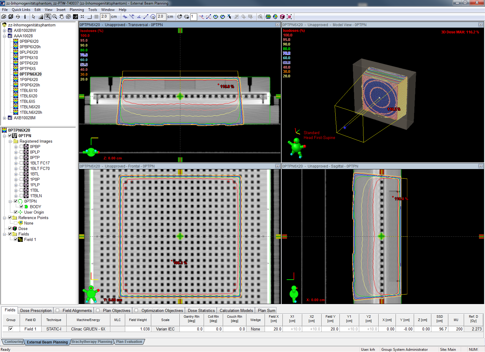
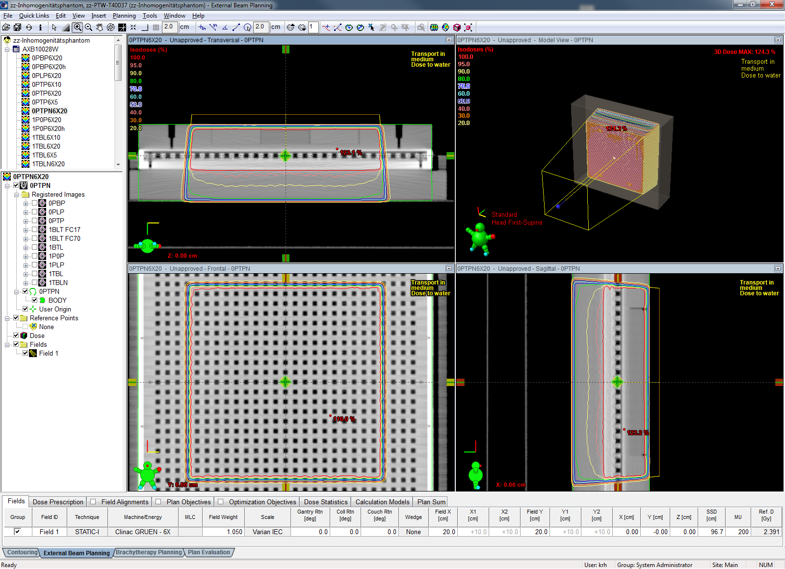
The kUser factors were determined for a grid size of 2.5 mm and the setup 0PTP, which stands for PMMA, Tissue, PMMA and no extra buildup. This is the most homogeneous setup acheivable with the T40037 phantom. Temperature and pressure were corrected during the measurement, therefore kUser is sort of residual k factor. Since the OCTAVIUS Detector has a Cobalt calibration, correction factors for beam quality etc. are contained in kUser, which should not be too different from 1. Moreover, the kUser factors should be similar for AAA and AXB.
We determined the three kUser factors k(AAA) = 0.988, k(AXB, D2M) = 0.988 for dose to medium, and k(AXB, D2W) = 0.999 for dose to water.
AAA 10.0.28
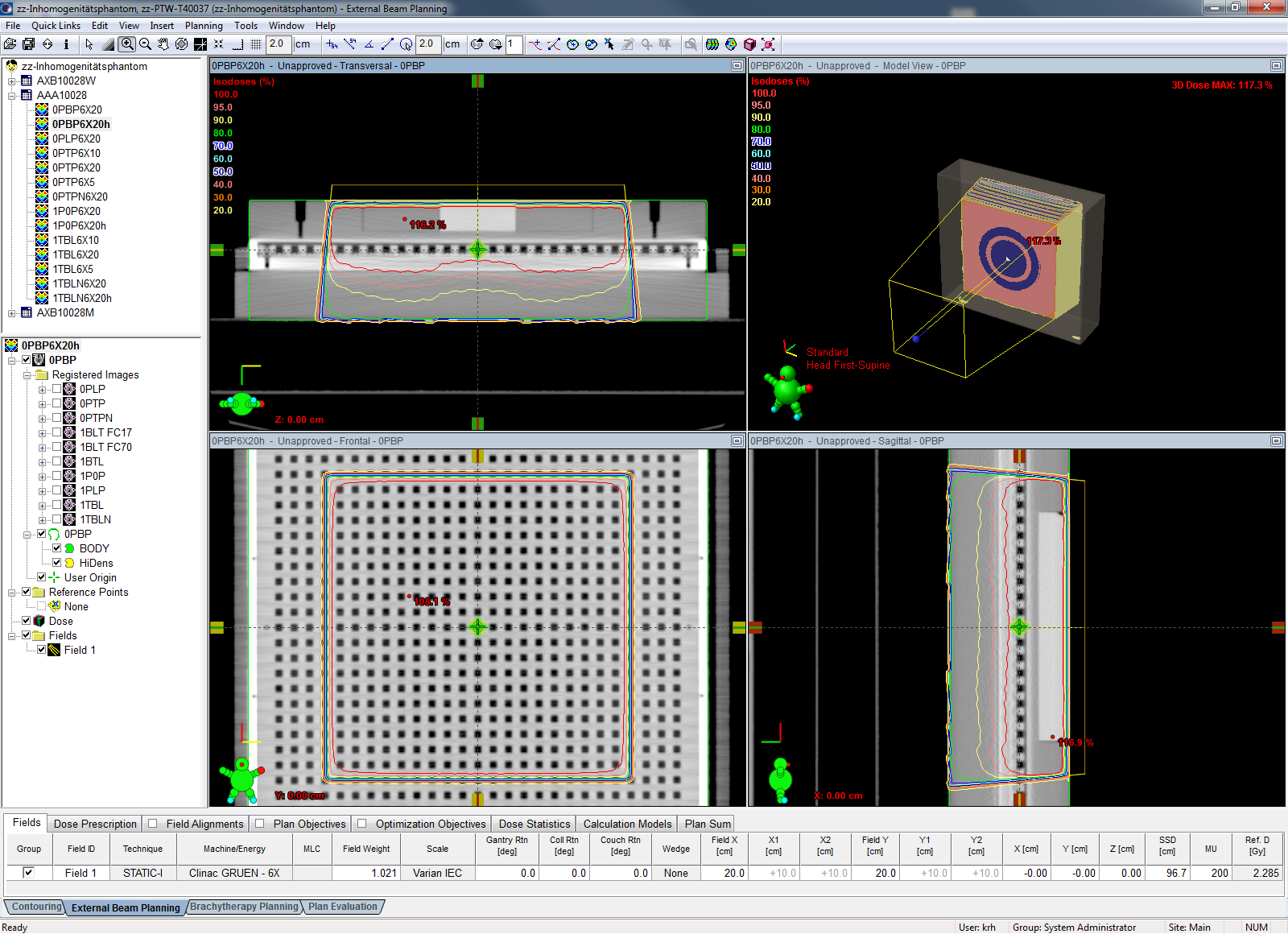
Since Acuros shall be compared to the established AAA, we first want to present the results of this algorithm. Screenshots of calculated isodoses can be found in column two (in Eclipse, 100% correspond to 2 Gy). The results in the last two columns are linked to the respective VeriSoft evaluation reports (PDFs):
| Measurement | AAA calculation | Grid [mm] | k(AAA) | GAI2,2[%] | GAI3,3[%] |
|---|---|---|---|---|---|
| 0PTP6X20d | 0PTPN6X20AAA(ref) | 2.5 | 0.988 | 91.6 | - |
| 1TBL6X20b | 1TBLN6X20AAA | 2.5 | 0.988 | 77.5 | 94.5 |
| 1TBL6X20b | 1TBLN6X20AAAh | 1.5 | 0.988 | - | 95.6 |
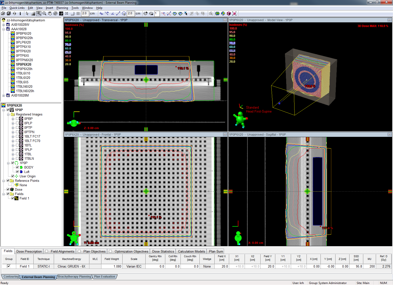
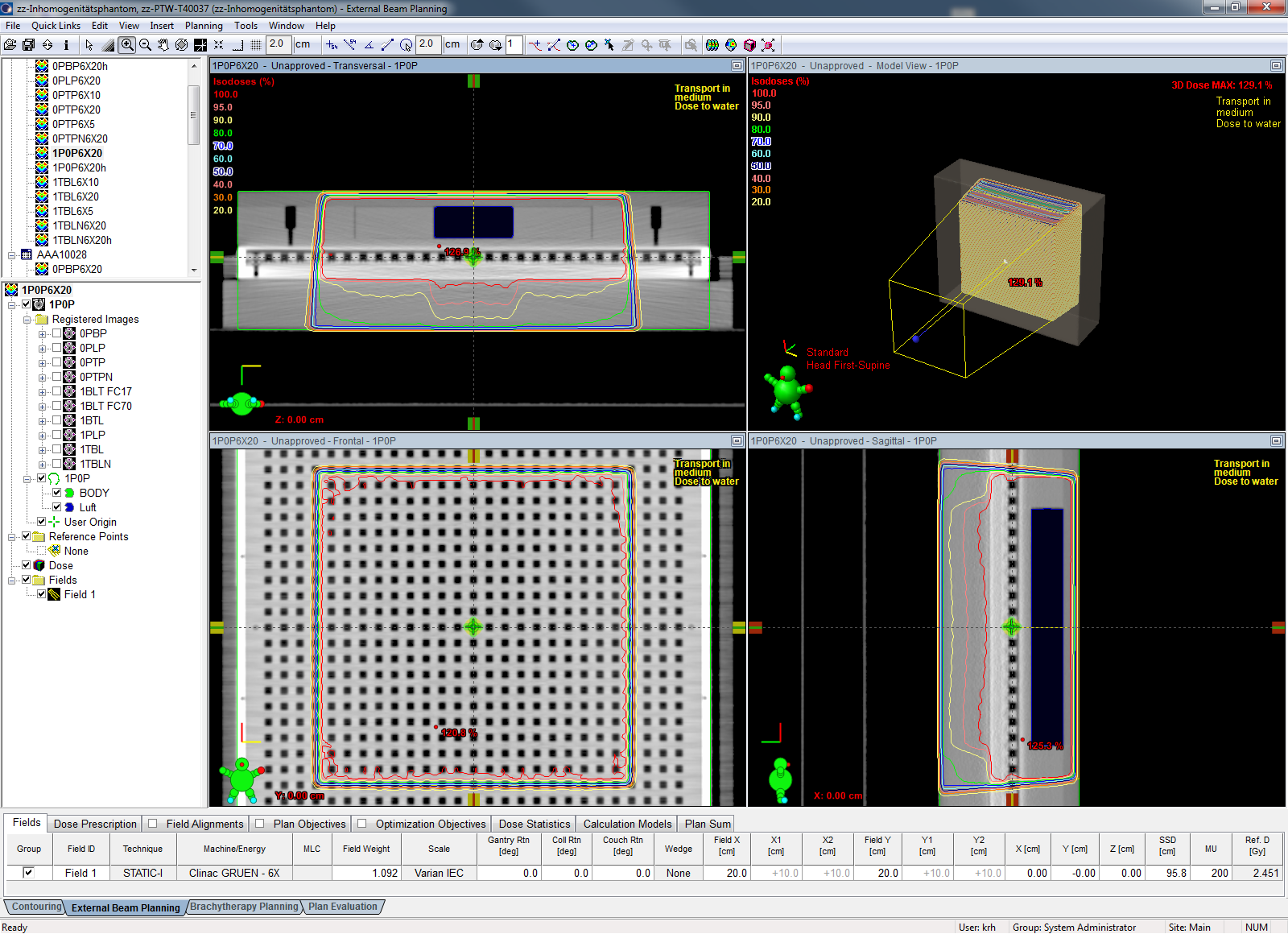
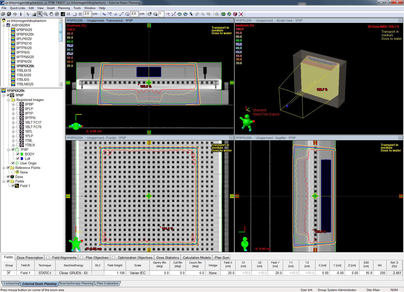
| 1P0P6X20b | 1P0P6X20AAA | 2.5 | 0.988 | 78.6 | 95.3 |
| 1P0P6X20b | 1P0P6X20AAAh | 1.5 | 0.988 | 92.0 | 96.2 |
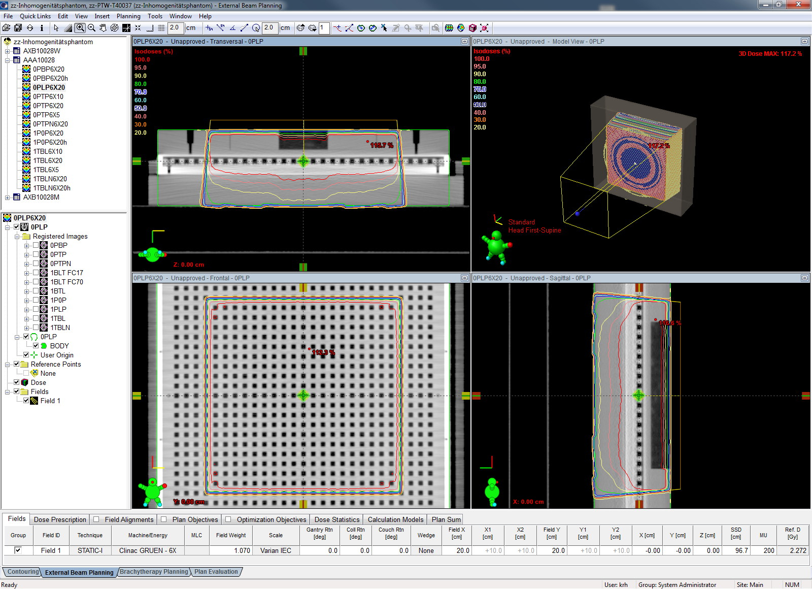
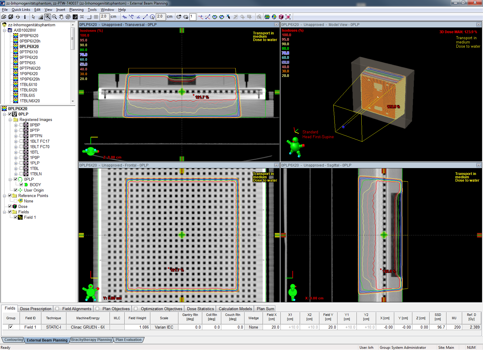
| 0PLP6X20a | 0PLP6X20AAA | 2.5 | 0.988 | 79.3 | - |
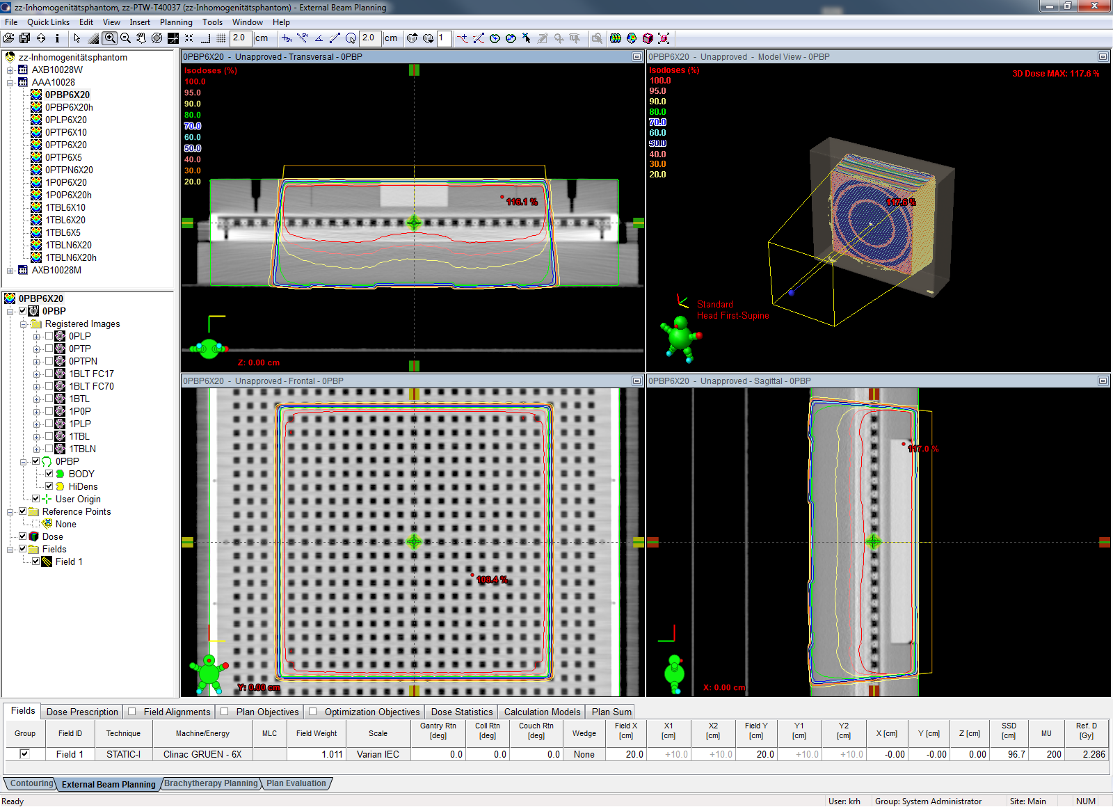
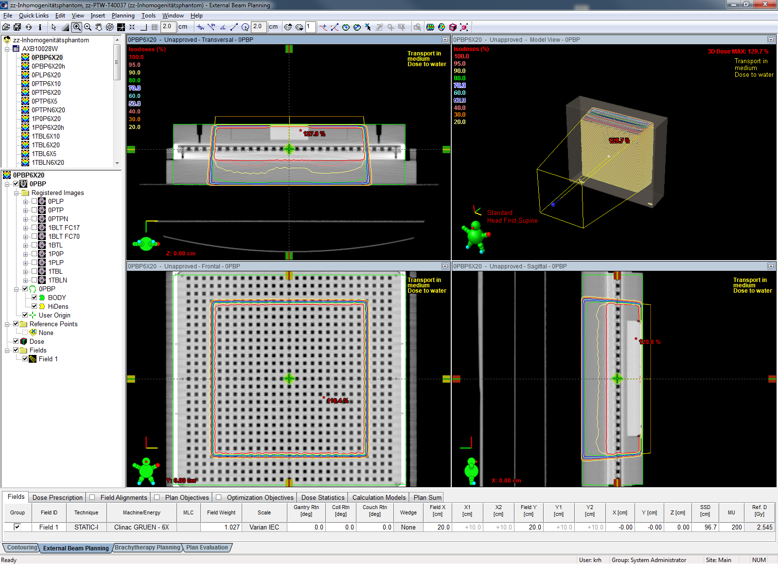
| 0PBP6X20b | 0PBP6X20AAA | 2.5 | 0.988 | 88.9 | 97.8 |
| 0PBP6X20b | 0PBP6X20AAAh | 1.5 | 0.988 | - | 92.6 |
Notes:
- The measurements were repeated several times, until reproducible results were achieved.
- The "N" in the first three AAA calculations stands for "native". It was first attempted to "mask" the 2D-Array's chambers with water in the Eclipse calculation, and the letter N distinguished between "masked" and "unmasked" calculations. It turned out that in the presence of inhomogeneities, masking is counterproductive and leads to large differences of kUser factors for the three algorithms (e.g. the masked AAA reference gave k(AAA) = 1.000, but k(AXB, D2M) = 0.939 and k(AXB, D2W) = 0.969. After giving up masking, kUser - differences between AAA and AXB(D2M) were gone.
- The maps of "failed points" in the PDF reports reveal that due to the limited spatial resolution of the 2D-Array, failed points often appear in the penumbra regions of the 20x20 field. This clearly has less significance for the tests like points that fail in the center of the field.
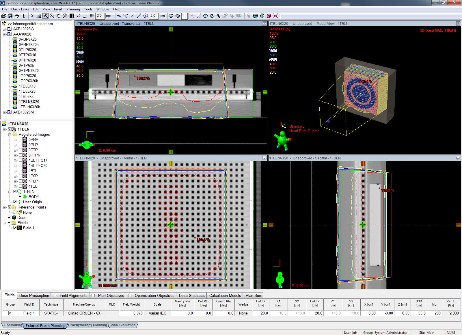
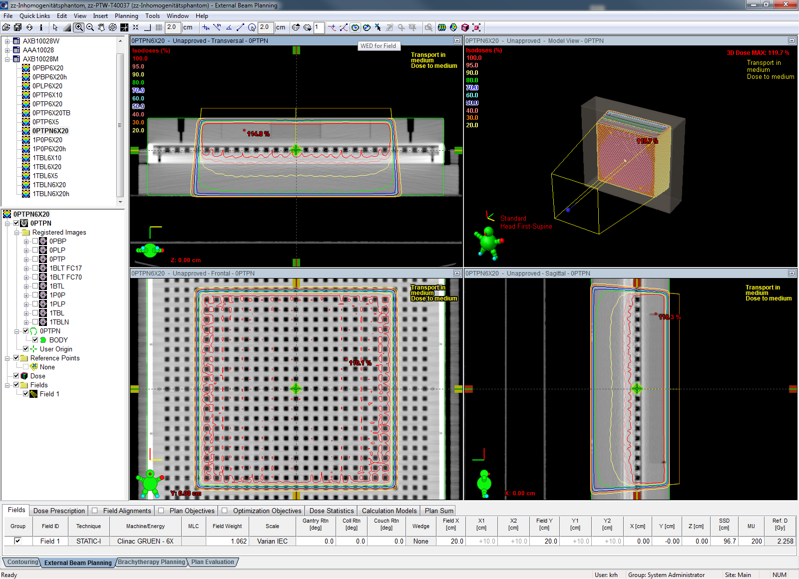
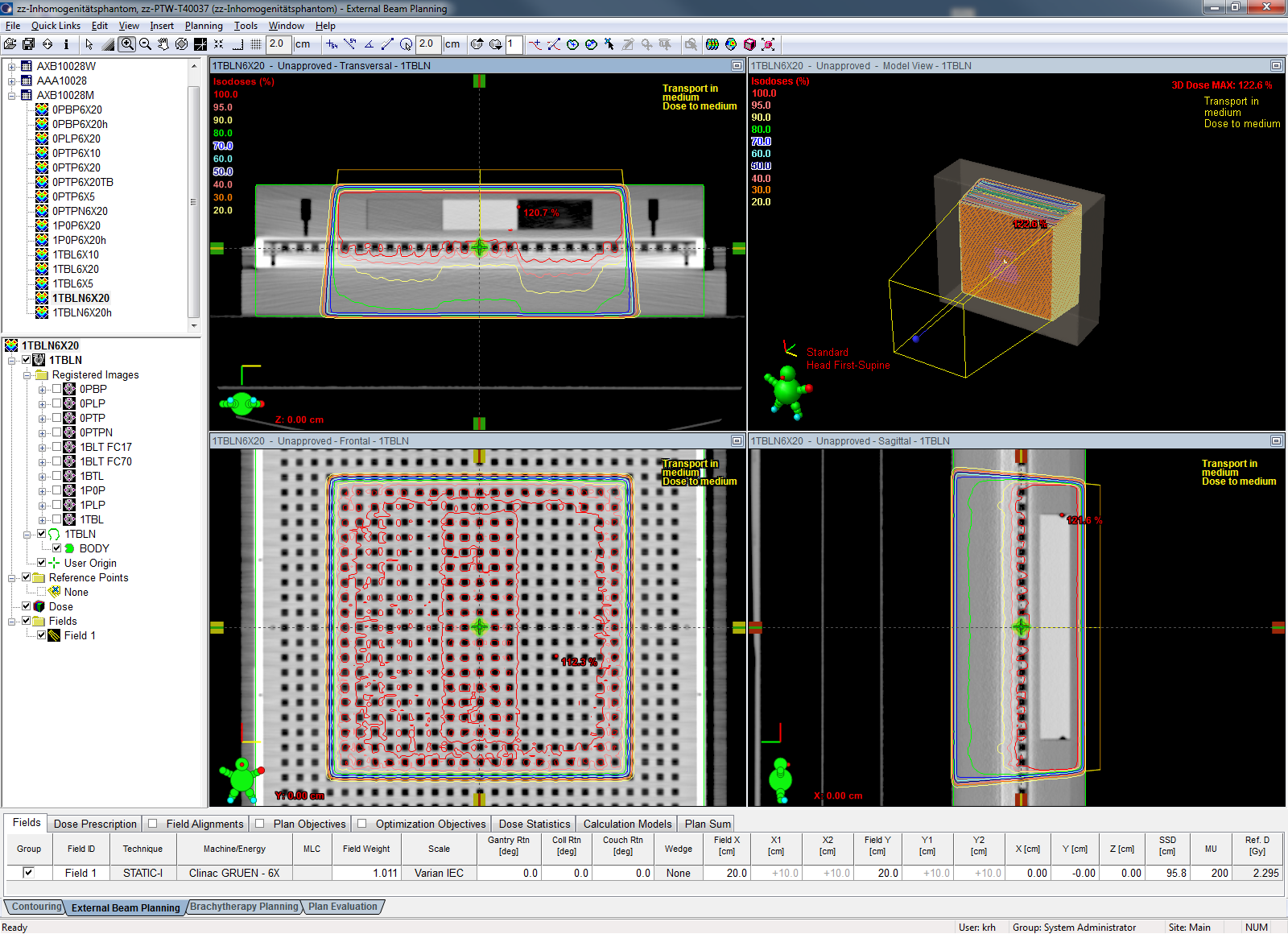
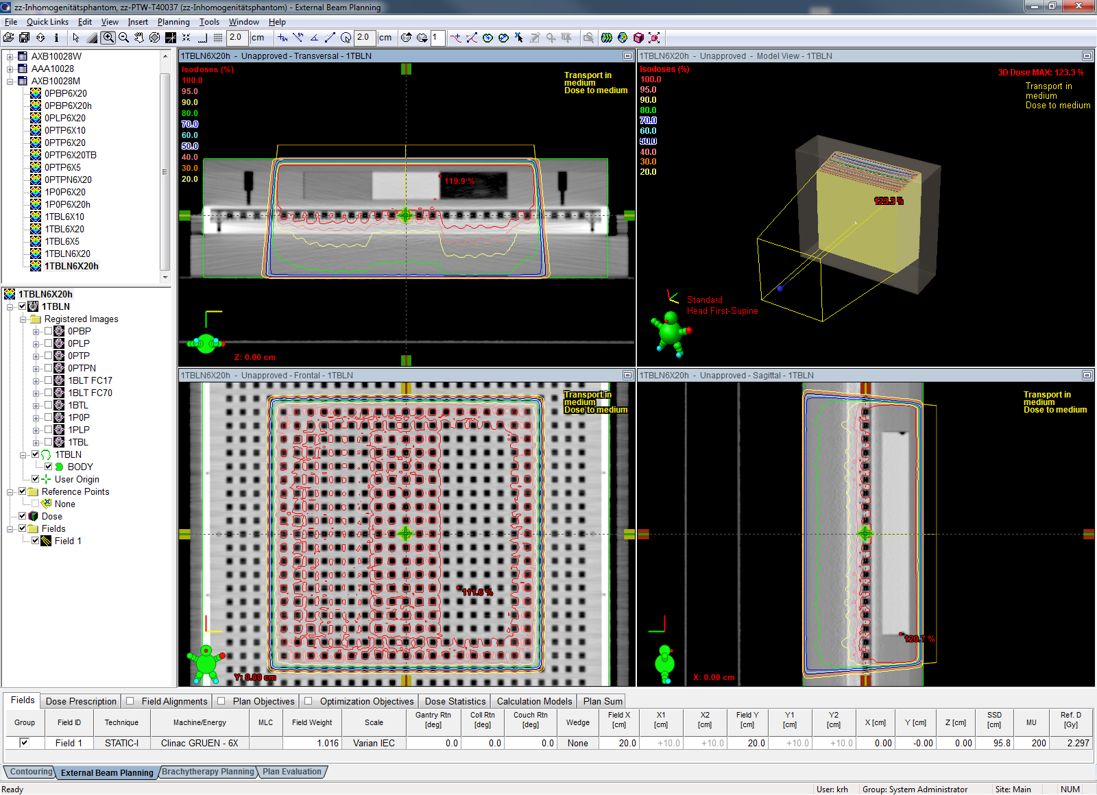
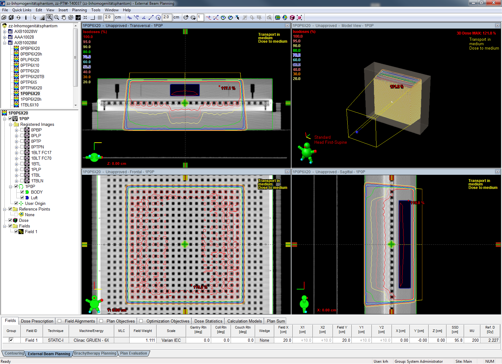
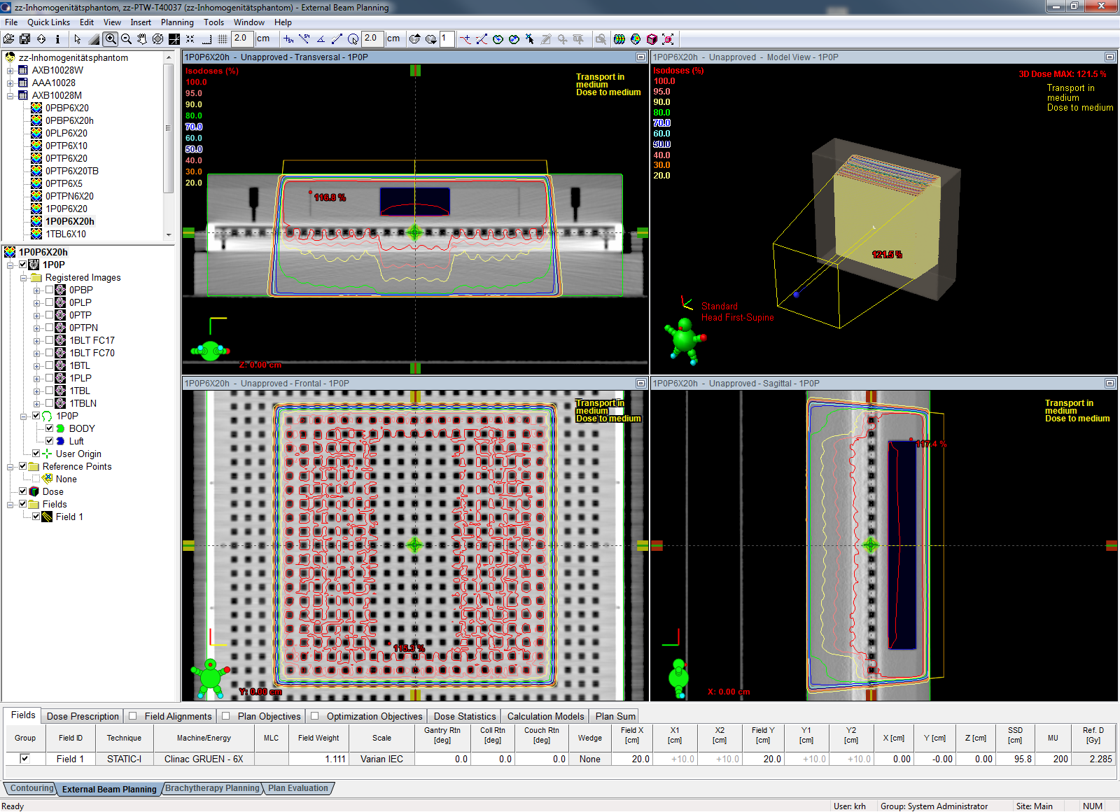
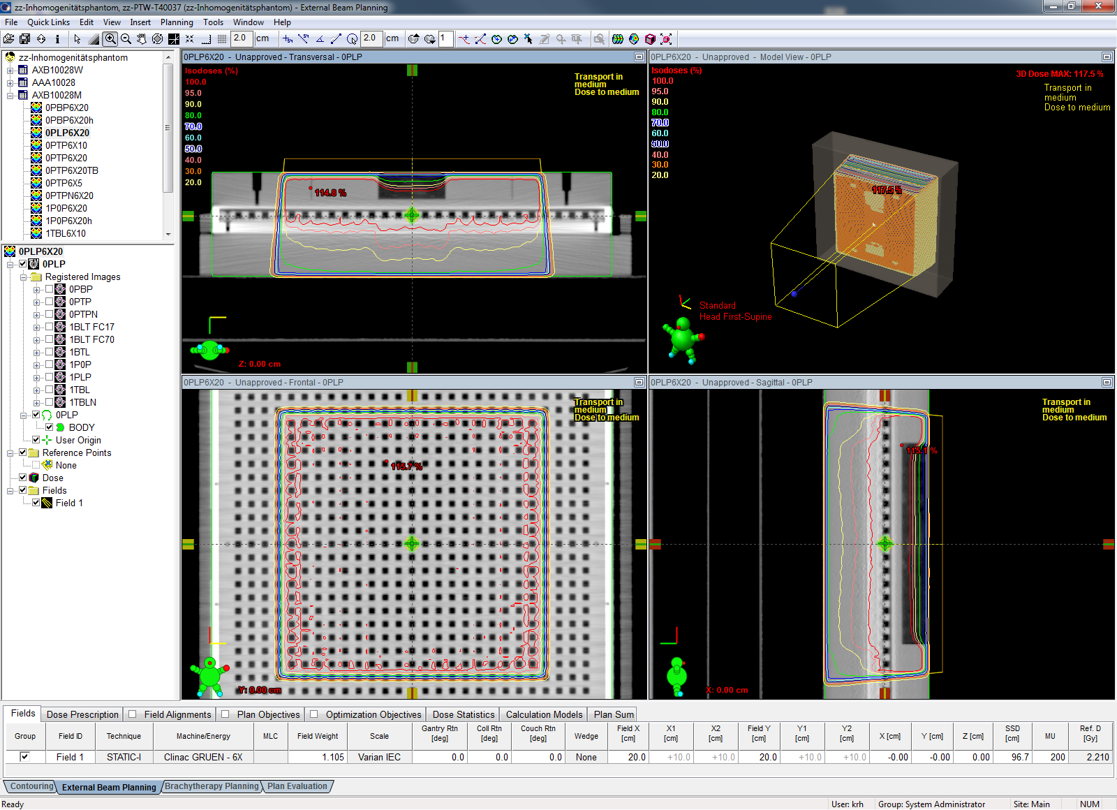
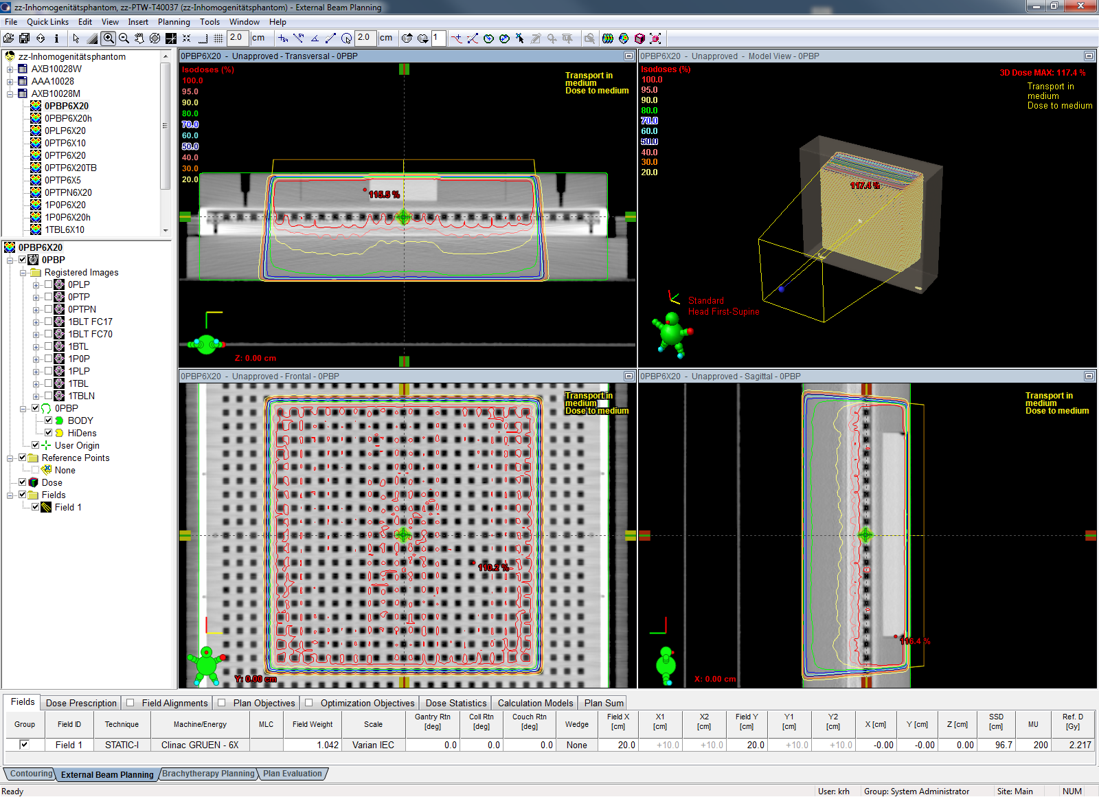
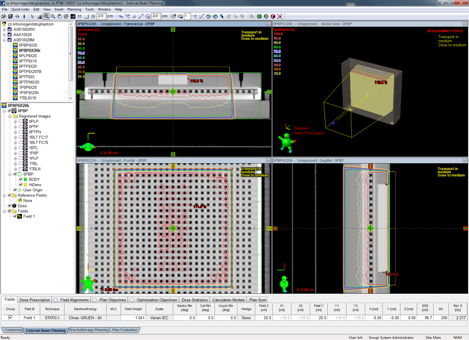
AcurosXB 10.0.28, reporting mode "Dose to medium"
The Acuros isodoses look rather different from the AAA isodoses, especially in regions of low density. The overall agreement with measurement (GAI) is generally better than for AAA. For the AXB(AAA), the average GAI2,2 = 85.9(84.65), the average GAI3,3 = 98.2(95.33):
| Measurement | AXB calculation (D2M) | Grid [mm] | k(AXB, D2M) | GAI2,2[%] | GAI3,3[%] |
|---|---|---|---|---|---|
| 0PTP6X20d | 0PTPN6X20AXB10M(ref) | 2.5 | 0.988 | 92.5 | - |
| 1TBL6X20b | 1TBLN6X20AXB10M | 2.5 | 0.988 | 82.3 | 99.3 |
| 1TBL6X20b | 1TBLN6X20AXB10Mh | 1.5 | 0.988 | - | 96.3 |
| 1P0P6X20b | 1P0P6X20AXB10M | 2.5 | 0.988 | 90.1 | 99.9 |
| 1P0P6X20b | 1P0P6X20AXB10Mh | 1.5 | 0.988 | 80.1 | 99.3 |
| 0PLP6X20a | 0PLP6X20AXB10M | 2.5 | 0.988 | 86.3 | - |
| 0PBP6X20b | 0PBP6X20AXB10M | 2.5 | 0.988 | 84.1 | 99.5 |
| 0PBP6X20b | 0PBP6X20AXB10Mh | 1.5 | 0.988 | - | 94.9 |
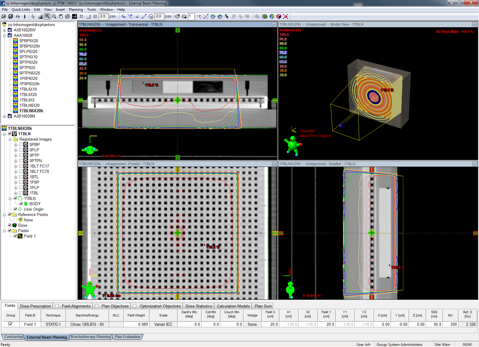
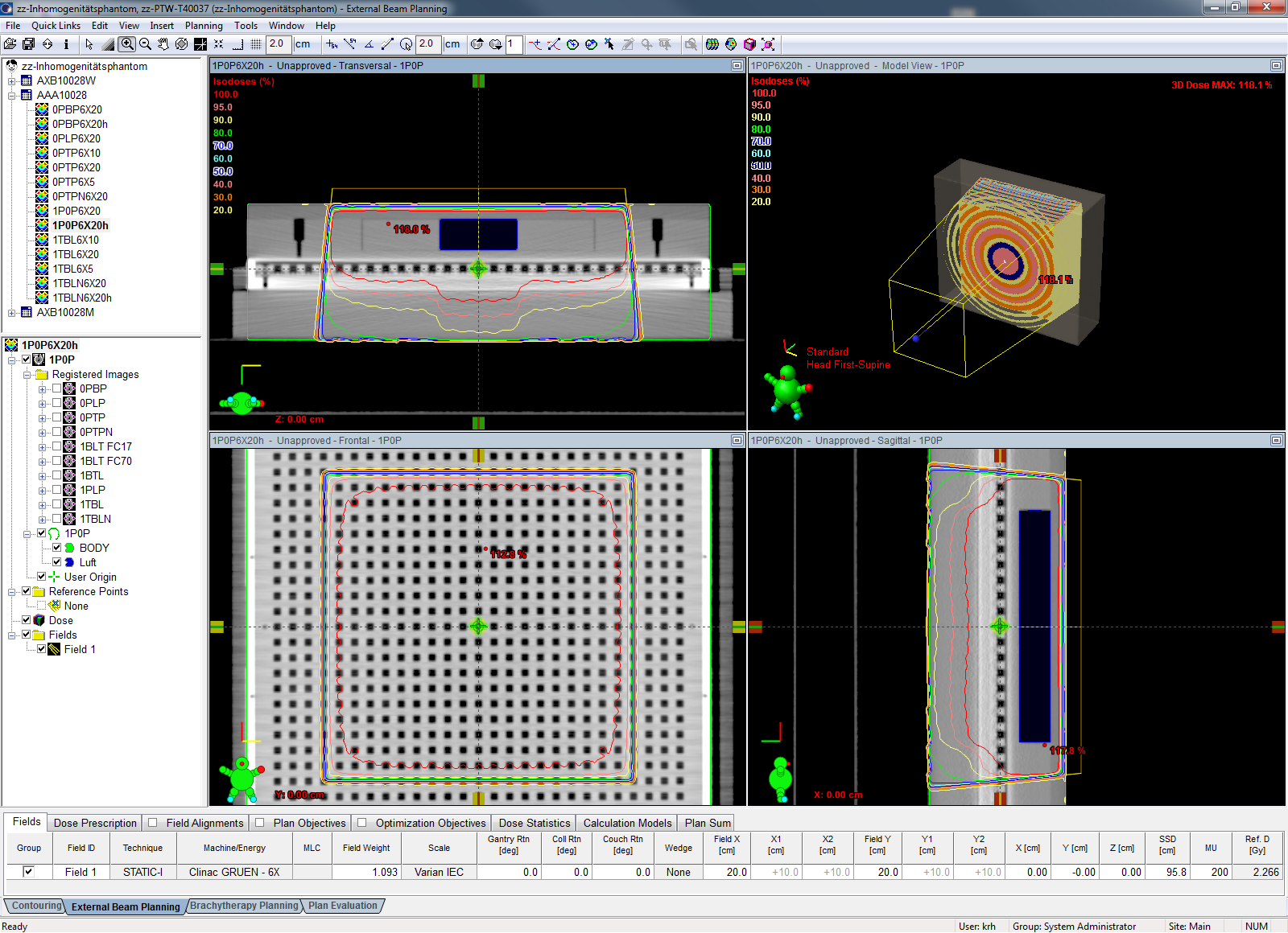
AcurosXB 10.0.28, reporting mode "Dose to water"
Whether treatment planning systems should report dose to medium or dose to water (or both) is a matter of debate since many years. For the D2W reporting mode, the agreement is somewhat better than for D2M, especially for the 2%/2mm criterion. If the same fields are compared (there are two more with GAI2,2 evaluations), the average GAI2,2 = 93.4, the average GAI3,3 = 98.9:
| Measurement | AXB calculation (D2W) | Grid [mm] | k(AXB, D2W) | GAI2,2[%] | GAI3,3[%] |
|---|---|---|---|---|---|
| 0PTP6X20d | 0PTPN6X20AXB10W(ref) | 2.5 | 0.999 | 91.9 | - |
| 1TBL6X20b | 1TBLN6X20AXB10W | 2.5 | 0.999 | 91.9 | 99.5 |
| 1TBL6X20b | 1TBLN6X20AXB10Wh | 1.5 | 0.999 | 85.6 | 98.5 |
| 1P0P6X20b | 1P0P6X20AXB10W | 2.5 | 0.999 | 95.5 | 99.0 |
| 1P0P6X20b | 1P0P6X20AXB10Wh | 1.5 | 0.999 | 94.9 | 98.8 |
| 0PLP6X20a | 0PLP6X20AXB10W | 2.5 | 0.999 | 91.5 | - |
| 0PBP6X20b | 0PBP6X20AXB10W | 2.5 | 0.999 | 92.6 | 99.7 |
| 0PBP6X20b | 0PBP6X20AXB10Wh | 1.5 | 0.999 | 89.7 | 97.8 |
Discussion
AcurosXB clearly performs better in the presence of inhomogeneities than AAA, at the expense of larger calculation times. D2W calculations show better agreement with measurements than D2M calculations.
One should remember that one key step of AXB is the material mapping. Phantoms made of PMMA with inserts made of Polystyrene ("Tissue") PTFE ("Bone") or some other plastic are by no means identical to real human tissue. The question now is, will a PTFE insert which gives 990 HU on the phantom CT scan produce the same radiation field as some real tissue with 990 HU? AXB only "sees" the HU coming from the CT, and maps them to real materials (tissues) with a certain chemical composition. This is a step which simply does not happen with AAA, and it could be the reason why D2W seems better than D2M, but in reality is not. We cannot know, because we can only measure in phantoms.
Now what should be the default dose reporting mode in Eclipse? One mode has to be selected as default, either D2M or D2W. Our current choice is D2M.